2. Calculate Turbidity from PRISM data#

BioSCape, the Biodiversity Survey of the Cape, is NASA’s first biodiversity-focused airborne and field campaign that was conducted in South Africa in 2023. BioSCape’s primary objective is to study the structure, function, and composition of the region’s ecosystems, and how and why they are changing.
BioSCape’s airborne dataset is unprecedented, with AVIRIS-NG, PRISM, and HyTES imaging spectrometers capturing spectral data across the UV, visible and infrared at high resolution and LVIS acquiring coincident full-waveform lidar. BioSCape’s field dataset is equally impressive, with 18 PI-led projects collecting data ranging from the diversity and phylogeny of plants, kelp and phytoplankton, eDNA, landscape acoustics, plant traits, blue carbon accounting, and more
This workshop will equip participants with the skills to find, subset, and visualize the various BioSCape field and airborne (imaging spectroscopy and full-waveform lidar) data sets. Participants will learn data skills through worked examples in terrestrial and aquatic ecosystems, including: wrangling lidar data, performing band math calculations, calculating spectral diversity metrics, spectral unmixing, machine learning and image classification, and mapping functional traits using partial least squares regression. The workshop format is a mix of expert talks and interactive coding notebooks and will be run through the BioSCape Cloud computing environment.
Date: October 9 - 11, 2024 Cape Town, South Africa
Host: NASA’s Oak Ridge National Laboratory Distributed Active Archive Center (ORNL DAAC), in close collaboration with BioSCape, the South African Environmental Observation Network (SAEON), the University of Wisconsin Madison (Phil Townsend), The Nature Conservancy (Glenn Moncrieff), the University of California Merced (Erin Hestir), the University of Cape Town (Jasper Slingsby), Jet Propulsion Laboratory (Kerry Cawse-Nicholson), and UNESCO.
Instructors:
In-person contributors: Anabelle Cardoso, Erin Hestir, Phil Townsend, Henry Frye, Glenn Moncrieff, Jasper Slingsby, Michele Thornton, Rupesh Shrestha
Virtual contributors: Kerry Cawse-Nicholson, Nico Stork, Kyle Kovach
Audience: This training is primarily intended for government natural resource management agency representatives and field technicians in South Africa, as well as local academics and students, especially those connected to the BioSCape Team.
2.1. Calculate Turbidity over a PRISM scene#
2.1.1. Overview#
Turbidity is a key water quality parameter that measures the clarity or cloudiness of water, primarily caused by the presence of suspended particles. These particles can include silt, clay, organic matter, algae, plankton, and other microscopic organisms. Essentially, turbidity indicates how much material is present in the water that scatters or absorbs light, which directly impacts its transparency.
 Water samples showing increasing turbidity and changes in water color. From https://blogs.worldbank.org/en/water/how-test-water-quality-here-are-some-low-cost-low-tech-options
As a water quality indicator, turbidity can reveal much about aquatic habitats. High turbidity can reduce light penetration, which affects photosynthesis in aquatic plants and algae. This reduction in primary productivity impacts the entire aquatic food web. High turbidity can also clog fish gills and reduce habitat quality for aquatic organisms. High turbidity often correlates with elevated nutrient levels, particularly phosphorus, which can promote excessive algal growth, leading to eutrophication. This process can deplete oxygen levels in the water, harming fish and other aquatic organisms. In some instances, moderate to high turbidity is necessary for certain fish species, as they are well-adapted for low light environments.
Additionally, turbidity is a critical parameter for drinking water quality. Elevated turbidity may indicate the presence of pathogens such as bacteria, viruses, and parasites, as these microorganisms can attach to suspended particles. Thus, clear water is generally considered safer for consumption.
The Portable Remote Imaging Spectrometer (PRISM) is especially designed for aquatic applications, and is well suited to measure water-leaving reflectance, which can be used to calculate turbidity. In this notebook, we will revisit opening a PRISM scene over the Theerwaterskloof Dam, the largest Dam in the province, accounting for 54% of the province’s water supply. The region experienced heavy rainfall during the winter and spring of 2023, leading to high river flows and filling the dam to 100% with overspilling by the end of September 2023.
2.1.2. Learning Objectives#
Mount the BioSCape SMCE S3 object storage in a local environment
Examine PRISM data using GDAL
Identify band numbers and associated wavelengths
Calculate turbidity using a single-band semi-empirical algorithm
Create and save a turbidity map as a GeoTIFF file
Visualize turbidity maps in QGIS
Compare two turbidity maps derived from two different wavelengths
2.1.3. Requirements#
import s3fs
import matplotlib.pyplot as plt
from osgeo import gdal
import numpy as np
import pandas as pd
from os import path
import rioxarray
gdal.UseExceptions()
2.1.4. Content#
Explore the BioSCape SMCE S3 PRISM data holdings Let’s start by exploring the BioSCape Airborne currently data available on the cloud in Amazon Storage. This AWS S3 storage is specific to the SMCE that provides data access and analytics environment to the BioSCape Science Team as well as interested researchers. We’ll learn how to mount the S3 object storage on our local environment, as well as learning how to bring other data to the analysis.
SMCE = Science Managed Cloud Environment S3 = Amazon Simple Storage Service (S3) is a cloud storage service that allows users to store and retrieve data S3Fs is a Pythonic open source tool that mounts S3 object storage locally. S3Fs provides a filesystem-like interface for accessing objects on S3. The top-level class S3FileSystem holds connection information and allows typical file-system style operations like ls ls is a UNIX command to list computer files and directories
# Use S3Fs to list the BioSCape data on the BioSCape SMCE S3 storage
s3 = s3fs.S3FileSystem(anon=False)
files = s3.ls('bioscape-data/')
files
['bioscape-data/AVNG',
 'bioscape-data/BioSCapeVegPolys2023_10_18',
 'bioscape-data/BioSCapeVegPolys2023_10_18.geoparquet',
 'bioscape-data/LVIS',
 'bioscape-data/PRISM',
 'bioscape-data/bioscape_avng.yaml']
2.1.4.1. Portable Remote Imaging Spectrometer (PRISM)#
PRISM_flightlines = s3.ls('bioscape-data/PRISM')
PRISM_flightlines
['bioscape-data/PRISM/L2']
Examine PRISM Reflectance Data as a GDAL Raster Dataset GDAL (Geospatial Data Abstraction Library) is a translator library for raster and vector geospatial data formats In this step, we will use GDAL to examine the PRISM reflectance data that is in ENVI binary format (a proprietary, but common distribution format)
We need to configure our S3 credentials for GDAL The GDAL utility expects S3 links to be formated with the GDAL virtual file system (VSI) S3 path. We therefore have to use the VSI path to access the files with GDAL. We’ll substitute the S3 link with the VSI (vsis3) link(s).
rfl_link = 'bioscape-data/PRISM/L2/prm20231126t080430_rfl_ort'
image_open = gdal.Open(path.join('/vsis3', rfl_link))
#image_open.GetMetadata()
# lists of band numbers and band center
band_numbers = [int(b.split("_")[1]) for b in image_open.GetMetadata().keys() if b != "wavelength_units"]
band_wavelength = [float(b.split(" ")[0]) for b in image_open.GetMetadata().values() if b != "Nanometers"]

# data frame describing bands
bands = pd.DataFrame({
    "Band number": band_numbers,
    "Band wavelength (nm)": band_wavelength}, index = band_wavelength).sort_index()

print(bands.to_string())
Band number Band wavelength (nm)
350.554829 1 350.554829
353.385086 2 353.385086
356.215399 3 356.215399
359.045768 4 359.045768
361.876193 5 361.876193
364.706675 6 364.706675
367.537213 7 367.537213
370.367807 8 370.367807
373.198457 9 373.198457
376.029164 10 376.029164
378.859927 11 378.859927
381.690746 12 381.690746
384.521621 13 384.521621
387.352553 14 387.352553
390.183541 15 390.183541
393.014585 16 393.014585
395.845685 17 395.845685
398.676841 18 398.676841
401.508054 19 401.508054
404.339323 20 404.339323
407.170649 21 407.170649
410.002030 22 410.002030
412.833468 23 412.833468
415.664962 24 415.664962
418.496512 25 418.496512
421.328118 26 421.328118
424.159781 27 424.159781
426.991500 28 426.991500
429.823275 29 429.823275
432.655106 30 432.655106
435.486994 31 435.486994
438.318938 32 438.318938
441.150938 33 441.150938
443.982994 34 443.982994
446.815107 35 446.815107
449.647276 36 449.647276
452.479501 37 452.479501
455.311782 38 455.311782
458.144120 39 458.144120
460.976514 40 460.976514
463.808964 41 463.808964
466.641470 42 466.641470
469.474033 43 469.474033
472.306651 44 472.306651
475.139326 45 475.139326
477.972058 46 477.972058
480.804845 47 480.804845
483.637689 48 483.637689
486.470589 49 486.470589
489.303545 50 489.303545
492.136557 51 492.136557
494.969626 52 494.969626
497.802751 53 497.802751
500.635932 54 500.635932
503.469169 55 503.469169
506.302463 56 506.302463
509.135813 57 509.135813
511.969219 58 511.969219
514.802681 59 514.802681
517.636200 60 517.636200
520.469775 61 520.469775
523.303406 62 523.303406
526.137093 63 526.137093
528.970837 64 528.970837
531.804637 65 531.804637
534.638493 66 534.638493
537.472405 67 537.472405
540.306373 68 540.306373
543.140398 69 543.140398
545.974479 70 545.974479
548.808616 71 548.808616
551.642810 72 551.642810
554.477060 73 554.477060
557.311366 74 557.311366
560.145728 75 560.145728
562.980146 76 562.980146
565.814621 77 565.814621
568.649152 78 568.649152
571.483739 79 571.483739
574.318382 80 574.318382
577.153082 81 577.153082
579.987838 82 579.987838
582.822650 83 582.822650
585.657518 84 585.657518
588.492443 85 588.492443
591.327424 86 591.327424
594.162461 87 594.162461
596.997554 88 596.997554
599.832704 89 599.832704
602.667910 90 602.667910
605.503172 91 605.503172
608.338490 92 608.338490
611.173865 93 611.173865
614.009295 94 614.009295
616.844782 95 616.844782
619.680325 96 619.680325
622.515925 97 622.515925
625.351581 98 625.351581
628.187293 99 628.187293
631.023061 100 631.023061
633.858885 101 633.858885
636.694766 102 636.694766
639.530703 103 639.530703
642.366696 104 642.366696
645.202745 105 645.202745
648.038851 106 648.038851
650.875013 107 650.875013
653.711231 108 653.711231
656.547505 109 656.547505
659.383836 110 659.383836
662.220223 111 662.220223
665.056666 112 665.056666
667.893165 113 667.893165
670.729721 114 670.729721
673.566333 115 673.566333
676.403001 116 676.403001
679.239725 117 679.239725
682.076505 118 682.076505
684.913342 119 684.913342
687.750235 120 687.750235
690.587185 121 690.587185
693.424190 122 693.424190
696.261252 123 696.261252
699.098370 124 699.098370
701.935544 125 701.935544
704.772774 126 704.772774
707.610061 127 707.610061
710.447404 128 710.447404
713.284803 129 713.284803
716.122258 130 716.122258
718.959770 131 718.959770
721.797338 132 721.797338
724.634962 133 724.634962
727.472642 134 727.472642
730.310379 135 730.310379
733.148172 136 733.148172
735.986021 137 735.986021
738.823926 138 738.823926
741.661888 139 741.661888
744.499906 140 744.499906
747.337980 141 747.337980
750.176110 142 750.176110
753.014297 143 753.014297
755.852539 144 755.852539
758.690838 145 758.690838
761.529194 146 761.529194
764.367605 147 764.367605
767.206073 148 767.206073
770.044597 149 770.044597
772.883177 150 772.883177
775.721813 151 775.721813
778.560506 152 778.560506
781.399255 153 781.399255
784.238060 154 784.238060
787.076921 155 787.076921
789.915839 156 789.915839
792.754813 157 792.754813
795.593843 158 795.593843
798.432929 159 798.432929
801.272072 160 801.272072
804.111271 161 804.111271
806.950526 162 806.950526
809.789837 163 809.789837
812.629205 164 812.629205
815.468629 165 815.468629
818.308109 166 818.308109
821.147645 167 821.147645
823.987237 168 823.987237
826.826886 169 826.826886
829.666591 170 829.666591
832.506353 171 832.506353
835.346170 172 835.346170
838.186044 173 838.186044
841.025974 174 841.025974
843.865960 175 843.865960
846.706002 176 846.706002
849.546101 177 849.546101
852.386256 178 852.386256
855.226467 179 855.226467
858.066734 180 858.066734
860.907058 181 860.907058
863.747438 182 863.747438
866.587874 183 866.587874
869.428366 184 869.428366
872.268915 185 872.268915
875.109520 186 875.109520
877.950181 187 877.950181
880.790898 188 880.790898
883.631672 189 883.631672
886.472502 190 886.472502
889.313388 191 889.313388
892.154330 192 892.154330
894.995328 193 894.995328
897.836383 194 897.836383
900.677494 195 900.677494
903.518662 196 903.518662
906.359885 197 906.359885
909.201165 198 909.201165
912.042501 199 912.042501
914.883893 200 914.883893
917.725341 201 917.725341
920.566846 202 920.566846
923.408407 203 923.408407
926.250024 204 926.250024
929.091697 205 929.091697
931.933427 206 931.933427
934.775213 207 934.775213
937.617055 208 937.617055
940.458953 209 940.458953
943.300908 210 943.300908
946.142919 211 946.142919
948.984986 212 948.984986
951.827109 213 951.827109
954.669289 214 954.669289
957.511525 215 957.511525
960.353817 216 960.353817
963.196165 217 963.196165
966.038569 218 966.038569
968.881030 219 968.881030
971.723547 220 971.723547
974.566121 221 974.566121
977.408750 222 977.408750
980.251436 223 980.251436
983.094178 224 983.094178
985.936976 225 985.936976
988.779830 226 988.779830
991.622741 227 991.622741
994.465708 228 994.465708
997.308731 229 997.308731
1000.151810 230 1000.151810
1002.994946 231 1002.994946
1005.838138 232 1005.838138
1008.681386 233 1008.681386
1011.524690 234 1011.524690
1014.368051 235 1014.368051
1017.211468 236 1017.211468
1020.054941 237 1020.054941
1022.898470 238 1022.898470
1025.742056 239 1025.742056
1028.585698 240 1028.585698
1031.429396 241 1031.429396
1034.273150 242 1034.273150
1037.116961 243 1037.116961
1039.960827 244 1039.960827
1042.804750 245 1042.804750
1045.648730 246 1045.648730
Take note of the band numbers and corresponding wavelengths. We will use this information later on.
# Open the PRISM ENVI file and read the file bands, row, cols
#image_open = gdal.Open(gdal_url)

nbands = image_open.RasterCount
nrows = image_open.RasterYSize
ncols = image_open.RasterXSize

print("\n".join(["Bands:\t"+str(nbands), "Rows:\t"+str(nrows), "Cols:\t"+str(ncols)]))
Bands:	246
Rows:	2789
Cols:	655
2.1.5. Calculate Turbidity#
We are going to use a simple, but globally validated single-band algorithm for turbidity developed by Nechad et al. (2010). It is a semi-empirical water-leaving reflectance based algorithm. It has been found to be particularly useful for coastal, estuarine, and inland waters. It uses the relationship between water-leaving reflectance and turbidity, relying on measurements from visible and near-infrared (NIR) spectral bands to quantify the concentration of suspended particulate matter (SPM).
Where \(R_{w}\) is the water-leaving reflectance at a given wavelength, and A and C are given below.
The algorithm typically uses red or NIR bands (e.g., around 645 nm or 858 nm). The choice of wavelength depends on the water type; for example, red bands are generally used in relatively clear waters, while NIR bands are more suitable for highly turbid waters. As you have observed, as turbidity, or SPM, increases, water-leaving reflectance tends to increase, and peak reflectance tends to shift to longer wavelengths.
The coefficients \(A\) and \(C\) are empirically derived through in-situ measurements of turbidity and corresponding remote sensing data, which helps in tuning the model for different environments. In this example, we will use parameters taken from Dogliotti et al. 2011.
We are going to implement the algorithm on two wavelengths, and we will compare the results.
Wavelength |
PRISM band |
A |
C |
|---|---|---|---|
645 nm |
105 |
228.1 |
0.1641 |
858 nm |
180 |
3078.9 |
0.2112 |
2.1.5.1. Using GDAL to read a raster file as a numerical array#
convert an existing Gdal Dataset or a Band into a numpy array with the ReadAsArray() function
img_red = image_open.GetRasterBand(105).ReadAsArray()  # Band 105 is 645nm
img_nir = image_open.GetRasterBand(180).ReadAsArray()  # Band 181 is 858nm
# Calculate Turbidity

# Define the function T
def T(A, C, Rw):
    return (A * Rw) / (1 - (Rw / C))

turb_red = T(228.1, 0.1641, img_red)
turb_nir = T(3078.9, 0.2112, img_nir)
2.1.5.2. Explore the Results#
# Compare turbidity values of two different aquatic plots
# Note here when we print an element in a numpy array, the order is row column

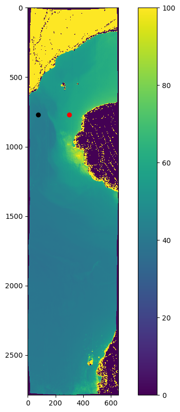
pixel1 = turb_red[770, 300] #  pixel location: row, col
pixel2 = turb_red[770, 75] # pixel location: row, col

print("The turbidity (645 nm) value at pixel 1 is " + str(pixel1))
print("The turbidity (645 nm) value at pixel 2 is " + str(pixel2))
The turbidity (645 nm) value at pixel 1 is 40.846443
The turbidity (645 nm) value at pixel 2 is 25.71505
pixel3 = turb_nir[770, 300] #  pixel location: row, col
pixel4 = turb_nir[770, 75] # pixel location: row, col

print("The turbidity (858 nm) value at pixel 3 is " + str(pixel3))
print("The turbidity (858 nm) value at pixel 4 is " + str(pixel4))
The turbidity (858 nm) value at pixel 3 is 59.01046
The turbidity (858 nm) value at pixel 4 is 41.42754
plt.scatter(300,770, color='red')
plt.scatter(75,770, color='black')
plt.rcParams['figure.figsize'] = [10,10]
plt.rcParams['figure.dpi'] = 100
#plt.imshow(turb_red, vmin=0, vmax=100) # not run
plt.imshow(turb_nir, vmin=0, vmax=100)
plt.colorbar()
plt.show()

2.1.6. Export turbidity maps as a stacked projected geoTIFFs#
img_red = image_open.GetRasterBand(105).ReadAsArray()  # Band 105 is 645nm red
img_nir = image_open.GetRasterBand(181).ReadAsArray()  # Band 70 is 860nm nir

outfile = ('prism_turbidity.tif')
rows = image_open.RasterYSize
cols = image_open.RasterXSize
datatype = image_open.GetRasterBand(1).DataType
projection = image_open.GetProjection()
transform = image_open.GetGeoTransform()

driver = gdal.GetDriverByName("GTiff")
DataSetOut = driver.Create(outfile, cols, rows, 2, datatype) # 2 band stack
DataSetOut.GetRasterBand(1).WriteArray(turb_red) # note the order of the band stack
DataSetOut.GetRasterBand(2).WriteArray(turb_nir)
DataSetOut.SetProjection(projection)
DataSetOut.SetGeoTransform(transform)
DataSetOut = None
2.1.6.1. Open QGIS in the Hub Desktop,#
From a Launcher tab, start the Desktop
At the bottom of the Desktop screen, use the Application Finder to find and launch QGIS
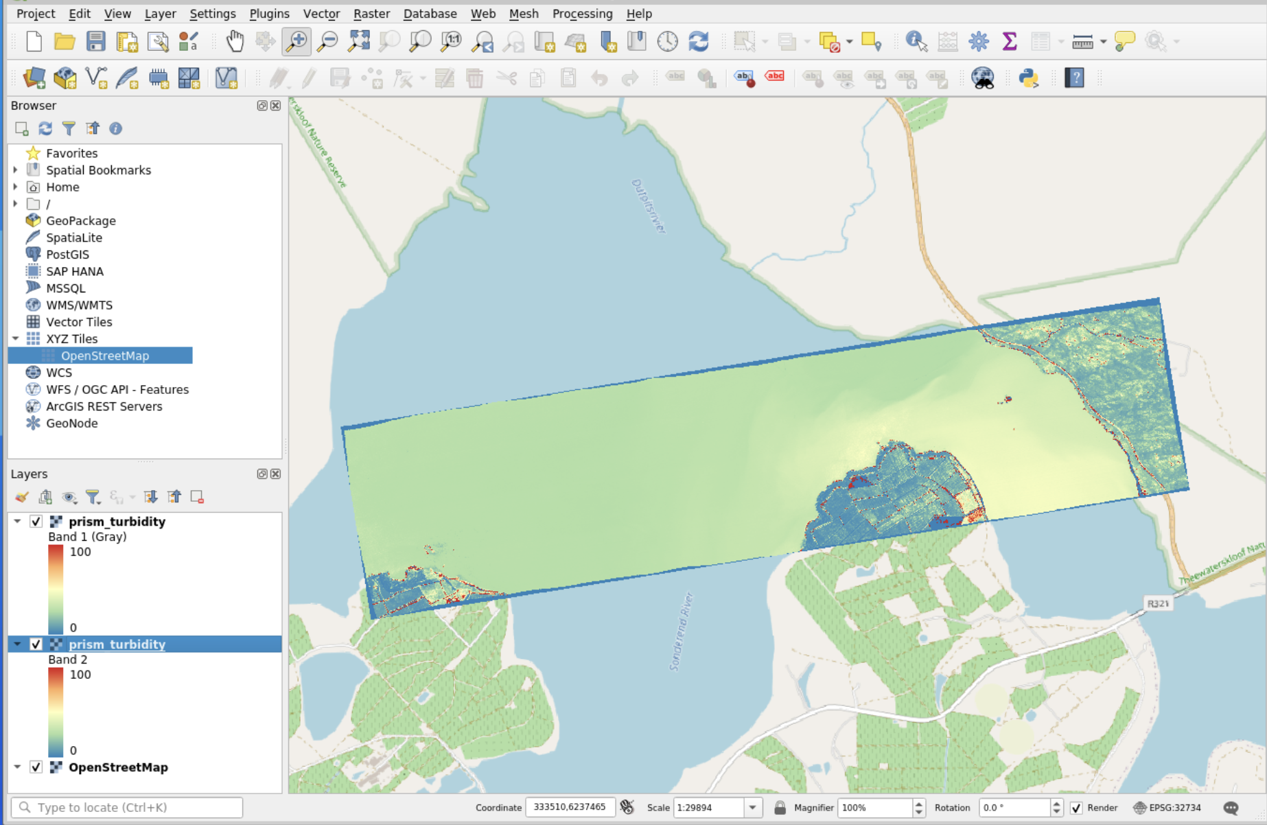
Using the Home file system, maneuver to the correct file folder containing the prism_turbidity.tif file, and view the prism_turbidity.tif image you just created !
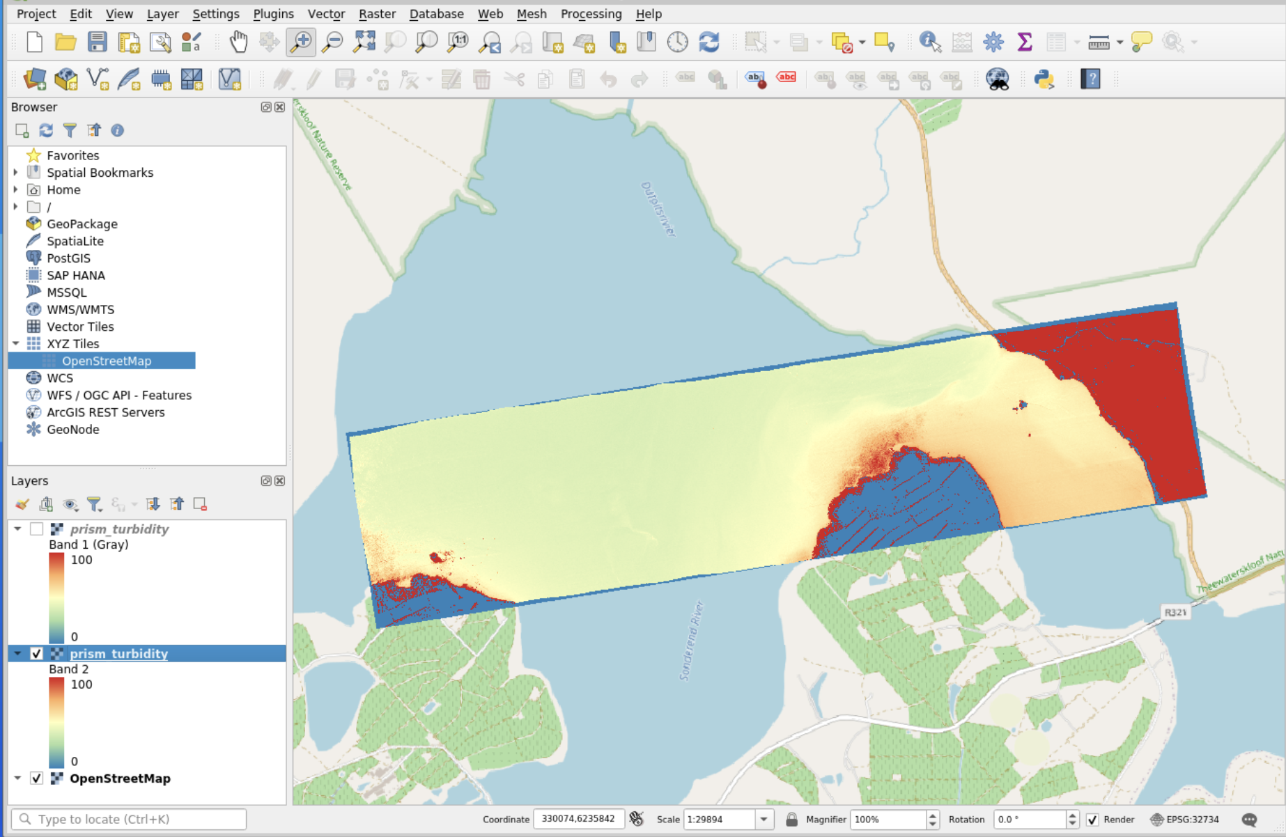
Note that we have created a two-band image. We can visualize each band to compare the two retrievals.
Load band 1 (turbidity from the red band)
Duplicate the layer and load band 2 (turbidity from the nir band)
HINT: under Symbology, set the Min/Max Value Settings to 0-100 so we are comparing the same scale
HINT: under Transparency, set the NoData value to 0


a copy of the output prism_turbidity.tif file is in the workshop folder
//shared/users/bioscape_ZA24workshop_data/RS_data/PRISM_Notebook

