Extract, Export to CSV, and Visualize Vegetation Plot Reflectance from AVIRIS-NG

5. Extract, Export to CSV, and Visualize Vegetation Plot Reflectance from AVIRIS-NG#

5.1. BioSCape Data Skills Workshop: From the Field to the Image#

Bioscape

BioSCape, the Biodiversity Survey of the Cape, is NASA’s first biodiversity-focused airborne and field campaign that was conducted in South Africa in 2023. BioSCape’s primary objective is to study the structure, function, and composition of the region’s ecosystems, and how and why they are changing.

BioSCape’s airborne dataset is unprecedented, with AVIRIS-NG, PRISM, and HyTES imaging spectrometers capturing spectral data across the UV, visible and infrared at high resolution and LVIS acquiring coincident full-waveform lidar. BioSCape’s field dataset is equally impressive, with 18 PI-led projects collecting data ranging from the diversity and phylogeny of plants, kelp and phytoplankton, eDNA, landscape acoustics, plant traits, blue carbon accounting, and more

This workshop will equip participants with the skills to find, subset, and visualize the various BioSCape field and airborne (imaging spectroscopy and full-waveform lidar) data sets. Participants will learn data skills through worked examples in terrestrial and aquatic ecosystems, including: wrangling lidar data, performing band math calculations, calculating spectral diversity metrics, machine learning and image classification, and mapping functional traits using partial least squares regression. The workshop format is a mix of expert talks and interactive coding notebooks and will be run through the BioSCape Cloud computing environment.

Date: October 9 - 11, 2024 Cape Town, South Africa

Host: NASA’s Oak Ridge National Laboratory Distributed Active Archive Center (ORNL DAAC), in close collaboration with BioSCape, the South African Environmental Observation Network (SAEON), the University of Wisconsin Madison (Phil Townsend), The Nature Conservancy (Glenn Moncrieff), the University of California Merced (Erin Hestir), the University of Cape Town (Jasper Slingsby), Jet Propulsion Laboratory (Kerry Cawse-Nicholson), and UNESCO.

Instructors:

In-person contributors: Anabelle Cardoso, Erin Hestir, Phil Townsend, Henry Frye, Glenn Moncrieff, Jasper Slingsby, Michele Thornton, Rupesh Shrestha
Virtual contributors: Kerry Cawse-Nicholson, Nico Stork, Kyle Kovach

Audience: This training is primarily intended for government natural resource management agency representatives and field technicians in South Africa, as well as local academics and students, especially those connected to the BioSCape Team.

5.2. Overview#

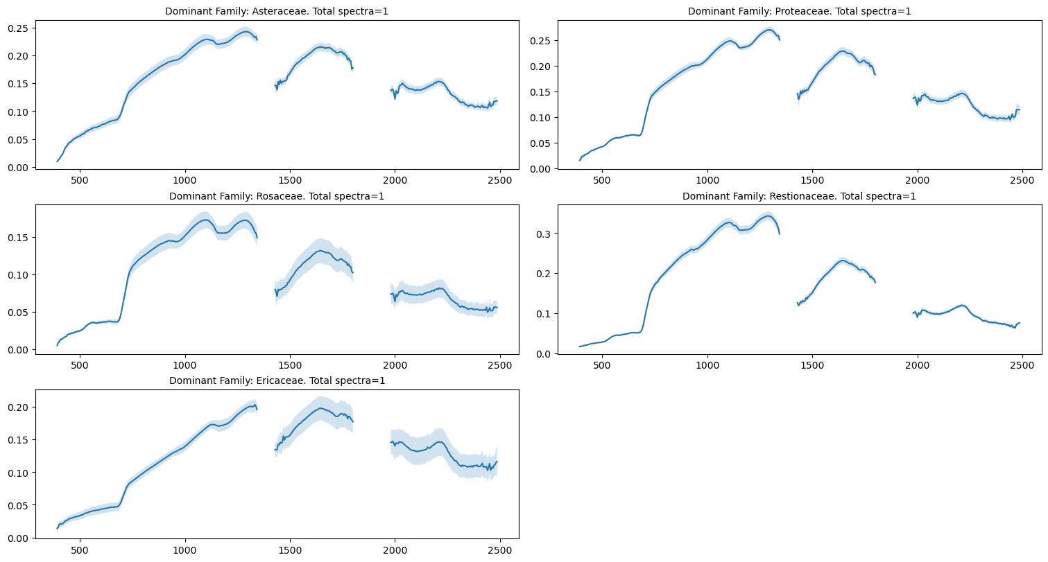
This tutorial will explore, discover, plot, and export to csv AVIRIS-NG spectral data for vegetation plot locations. In addition, for each plot location, a 3x3 pixel block of spectral data will be extracted and graphed by mean and standard deviation.

5.2.1. Learning Objectives#

Obtain the x,y values of the vegetation plot centers of interest
Determine which AVIRIS-NG scene corresponds to each of the vegetation center’s location
Extract and save the spectral values for each AVIRIS-NG band to a csv file for each vegetation center plot location
Extract the AVIRIS-NG spectral values for a 3x3 buffer around the center vegetation plot pixel
Graph the 3x3 mean and standard deviation

5.2.2. Load Python Modules#

# import python modules
from os import path
import numpy as np
import geopandas as gpd
import pandas as pd
import s3fs
import rioxarray
from pyproj import Proj
import matplotlib.pyplot as plt

# initialize S3 file system
s3 = s3fs.S3FileSystem(anon=False)

5.3. Read Vegetation centers#

The CapePeninsulaVegCenters.geojson contains the centroids of all vegetation plots within the Cape Peninsula region.

vegcenter = 'data/DominantFamPlotCenters.geojson'
v_gdf = gpd.read_file(vegcenter)
# keep only the columns we need
v_gdf = v_gdf[['BScpPID','Region','Name', 'QltyFlg', 'DominantFamily', 'geometry']]
print(f"total plots: {len(v_gdf.index)}")

total plots: 27

# subsetting to five plots of interest
v_gdf = v_gdf[v_gdf.BScpPID.isin(['T081', 'T093', 'T201', 'T069', 'T195'])]
v_gdf

	BScpPID	Region	Name	QltyFlg	DominantFamily	geometry
1	T093	CapePoint	CapePoint_93	None	Asteraceae	POINT (18.41285 -34.25000)
8	T081	CapePoint	CapePoint_81	None	Proteaceae	POINT (18.44767 -34.28852)
23	T069	capepoint	capepoint_69	None	Rosaceae	POINT (18.40220 -33.94848)
25	T195	capepoint	capepoint_195	None	Restionaceae	POINT (18.41104 -33.96294)
26	T201	capepoint	capepoint_201	None	Ericaceae	POINT (18.40614 -33.95935)

5.4. Read AVIRIS-NG Bounding Polygons#

The ANG_Coverage.geojson file contains two columns fid and scid which will help us identify the AVIRIS-NG granules and their folder structure.

ang_cov = 'data/ANG_Coverage.geojson'
a_gdf = gpd.read_file(ang_cov)
# keep only the columns we need
a_gdf = a_gdf[['fid', 'scid', 'start_time', 'geometry']]
a_gdf['start_time'] = pd.to_datetime(a_gdf['start_time']) # formatting start_time
a_gdf.head()

	fid	scid	start_time	geometry
0	ang20231022t092801	ang20231022t092801_000	2023-10-22 09:28:01+00:00	POLYGON ((18.75671 -32.94696, 18.79830 -32.945...
1	ang20231022t092801	ang20231022t092801_001	2023-10-22 09:28:01+00:00	POLYGON ((18.76213 -32.97934, 18.80428 -32.977...
2	ang20231022t092801	ang20231022t092801_002	2023-10-22 09:28:01+00:00	POLYGON ((18.76979 -33.01113, 18.81188 -33.009...
3	ang20231022t092801	ang20231022t092801_003	2023-10-22 09:28:01+00:00	POLYGON ((18.77388 -33.04254, 18.81612 -33.041...
4	ang20231022t092801	ang20231022t092801_004	2023-10-22 09:28:01+00:00	POLYGON ((18.77544 -33.07394, 18.81786 -33.072...

5.5. Get AVIRIS-NG spectra for each vegetation center coordinates#

We will retrieve AVIRIS-NG spectra of the center veg plot coordinates and save it as a CSV file.

First, find the vegetation points that are within the AVIRIS-NG polygons.

# spatial join of the veg plots and the ANG polygons dataframes
veg_ang_df = gpd.sjoin(v_gdf, a_gdf, predicate = 'within')
# adding X, Y columns
veg_ang_df['X'] = veg_ang_df.geometry.x
veg_ang_df['Y'] = veg_ang_df.geometry.y
# print
ang_plots_n = len(veg_ang_df.scid.unique())
ang_n = len(a_gdf.scid.unique())
print(f"{ang_plots_n} of {ang_n} AVIRIS-NG files overlaps with the veg plots")

16 of 9558 AVIRIS-NG files overlaps with the veg plots

We’ll narrow the AVIRIS-NG to scenes defined for this exercise

veg_ang_df = veg_ang_df[veg_ang_df.fid.str.startswith("ang20231109t13")]
veg_ang_df = veg_ang_df[veg_ang_df.fid != "ang20231109t130728"]
veg_ang_df

	BScpPID	Region	Name	QltyFlg	DominantFamily	geometry	index_right	fid	scid	start_time	X	Y
1	T093	CapePoint	CapePoint_93	None	Asteraceae	POINT (18.41285 -34.25000)	4193	ang20231109t133124	ang20231109t133124_003	2023-11-09 13:31:24+00:00	18.412845	-34.249997
8	T081	CapePoint	CapePoint_81	None	Proteaceae	POINT (18.44767 -34.28852)	4187	ang20231109t131923	ang20231109t131923_019	2023-11-09 13:19:23+00:00	18.447671	-34.288518
23	T069	capepoint	capepoint_69	None	Rosaceae	POINT (18.40220 -33.94848)	4203	ang20231109t133124	ang20231109t133124_013	2023-11-09 13:31:24+00:00	18.402198	-33.948477
25	T195	capepoint	capepoint_195	None	Restionaceae	POINT (18.41104 -33.96294)	4203	ang20231109t133124	ang20231109t133124_013	2023-11-09 13:31:24+00:00	18.411038	-33.962942
26	T201	capepoint	capepoint_201	None	Ericaceae	POINT (18.40614 -33.95935)	4203	ang20231109t133124	ang20231109t133124_013	2023-11-09 13:31:24+00:00	18.406135	-33.959346

Let’s first define two python functions.

def get_rfl_path(fid_str, scid_str):
    """returns s3 paths from fid and scid for aviris-ng files"""
    # list the ANG files
    a_fs = s3.ls(f'bioscape-data/AVNG/{fid_str}/{scid_str}')
    # loop through the file list and find the RFL file
    a_rfl = [a_f for a_f in a_fs if a_f.endswith("_RFL_ORT")][0]
    return path.join('s3://', a_rfl)

def subset_avirisng(rfl_xr, a_df):
    """returns a pandas dataframe with band names and spectral value 
    for a pixel"""
    # Proj class instance with AVN CRS. preserve_units false to ensure 
    # that input coordinates are in meters
    p = Proj(rfl_xr.rio.crs, preserve_units=False)
    # converts the lon,lat veg plot coordinates to the ANG map projection
    x, y = p(a_df.X, a_df.Y)
    # get the spectra of the ANG pixel nearest to the veg plot
    rfl_val = rfl_xr.sel(y=y, x=x, method='nearest').to_numpy()
    # get band names
    band_names = [f'Band_{i}' for i in a_rfl_xr.band.to_numpy()] 
    # convert band and spectra into a dataframe
    rfl_dict = dict(zip(band_names, rfl_val))
    rfl_df = pd.DataFrame([rfl_dict])  
     # add Name, scid columns which we will use to join dataframes later
    rfl_df['Name'] = a_df.Name
    rfl_df['scid'] = a_df.scid
    return rfl_df

Now, we can run the subsetting of AVIRIS-NG files over the vegetation plots.

# initialize a list for storing aviris dataframe
rfl_list = []
# total number of veg plots to process
sub_n = len(veg_ang_df.scid.unique())
# loop through AVNG files by scid
for i, scid in enumerate(veg_ang_df.scid.unique()):
    # get row(s) that matches scid
    a_temp_df = veg_ang_df[veg_ang_df['scid']==scid]
    # retrieve S3 path of the AVIRIS tile
    a_rfl = get_rfl_path(a_temp_df.fid.values[0], scid)
    print(f'reading scene {i+1} of {sub_n}: {path.basename(a_rfl)}')
    # open the RFL file
    a_rfl_xr = rioxarray.open_rasterio(a_rfl, drivers='ENVI', 
                                       chunks=True, parse_coordinates=True)
    # loop through the veg plots
    for s in a_temp_df.index:
        # get a row
        print(f'reading plot {s}')
        a_temp = a_temp_df.loc[s]       
        rfl_list.append(subset_avirisng(a_rfl_xr, a_temp))

# concatenate ANG spectra dataframe
avng_rfl_df = pd.concat(rfl_list)
# merge it with the a_sub_gdf dataframe
final_gdf = pd.merge(veg_ang_df, avng_rfl_df, on=["scid", "Name"], how="left")

reading scene 1 of 3: ang20231109t133124_003_L2A_OE_main_27577724_RFL_ORT
reading plot 1
reading scene 2 of 3: ang20231109t131923_019_L2A_OE_main_27577724_RFL_ORT
reading plot 8
reading scene 3 of 3: ang20231109t133124_013_L2A_OE_main_27577724_RFL_ORT
reading plot 23
reading plot 25
reading plot 26

final_gdf

	BScpPID	Region	Name	QltyFlg	DominantFamily	geometry	index_right	fid	scid	start_time	...	Band_416	Band_417	Band_418	Band_419	Band_420	Band_421	Band_422	Band_423	Band_424	Band_425
0	T093	CapePoint	CapePoint_93	None	Asteraceae	POINT (18.41285 -34.25000)	4193	ang20231109t133124	ang20231109t133124_003	2023-11-09 13:31:24+00:00	...	0.117443	0.105415	0.106884	0.109661	0.110175	0.110575	0.110969	0.111366	0.111767	-0.01
1	T081	CapePoint	CapePoint_81	None	Proteaceae	POINT (18.44767 -34.28852)	4187	ang20231109t131923	ang20231109t131923_019	2023-11-09 13:19:23+00:00	...	0.102414	0.096206	0.103456	0.105571	0.105515	0.105468	0.105377	0.105297	0.105204	-0.01
2	T069	capepoint	capepoint_69	None	Rosaceae	POINT (18.40220 -33.94848)	4203	ang20231109t133124	ang20231109t133124_013	2023-11-09 13:31:24+00:00	...	0.055511	0.056439	0.057473	0.062190	0.062239	0.062227	0.062194	0.062172	0.062154	-0.01
3	T195	capepoint	capepoint_195	None	Restionaceae	POINT (18.41104 -33.96294)	4203	ang20231109t133124	ang20231109t133124_013	2023-11-09 13:31:24+00:00	...	0.064210	0.064997	0.064468	0.067248	0.070095	0.071681	0.073924	0.075812	0.077774	-0.01
4	T201	capepoint	capepoint_201	None	Ericaceae	POINT (18.40614 -33.95935)	4203	ang20231109t133124	ang20231109t133124_013	2023-11-09 13:31:24+00:00	...	0.089417	0.095285	0.098122	0.104437	0.104813	0.105360	0.105832	0.106272	0.106747	-0.01

5 rows × 437 columns

5.5.1. The following will export the pandas dataframe to a CSV file.#

# write it to CSV
final_gdf.to_csv('ANG_RFL_CapePeninsulaVegCenters.csv', index=False)

5.5.1.1. ^^^ Open the csv file that just wrote to your File Browser. Just double click on the file name and it will open in a new tab.#

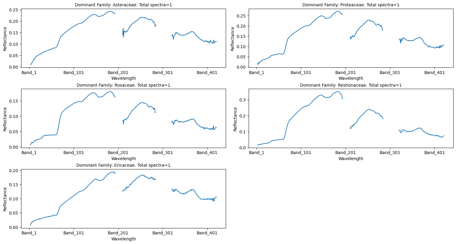
5.5.2. Create a spectral profile for each dominant family vegetation plot#

dominant = final_gdf.DominantFamily.unique()
fig = plt.figure(figsize=(15,8), constrained_layout=True)
columns = 2
rows = int(len(dominant)/columns)+1
for i, item in enumerate(dominant):
    # transpose and plot species
    dominant_df = final_gdf[final_gdf.DominantFamily == item]
    dominant_df = dominant_df.filter(like='Band')
    # drop rows with no data values
    dominant_df = dominant_df.replace(-9999, pd.NA).dropna()
    if not dominant_df.empty:
        # setting tails and atmospheric window to nan values
        dominant_df.iloc[:, np.r_[:3,194:210,285:320,422:425]] = np.nan
        dominant_n = len(dominant_df.index)
        ax = fig.add_subplot(rows, columns, i+1)
        dominant_df.T.plot(ax=ax, legend=None, 
                           xlabel="Wavelength", ylabel="Reflectance")
        # ax.set_xticks(a_rfl_xr.wavelength.values.tolist())
        ax.set_title(f"Dominant Family: {item}. Total spectra={len(dominant_df.index)}", 
                     fontsize=10)

plt.show()

5.6. Get AVIRIS-NG spectra for a buffer around the vegetation plot coordinates#

We will now retrieve AVIRIS-NG spectra of a 1-pixel buffer (3 x 3 pixels) around the center veg plot coordinates and save it as a CSV file.