BioSCape Campaign Overview
BioSCape: In October/November of 2023, the US National Aeronautics and Space Administration (NASA) conducted its first Biodiversity field and airborne campaign across terrestrial and aquatic environments in the South African Greater Cape Floristic Region (GCFR). From 4 airborne instruments;
Airborne Visible-Infrared Imaging Spectrometer - Next Generation (AVIRIS-NG),
Portable Remote Imaging SpectroMeter (PRISM),
Hyperspectral Thermal Emission Spectrometer (HyTES), and
Land, Vegetation, and Ice Sensor (LVIS),
the BioSCape Campaign’s remote sensing data products provide an unprecedented level of image spectroscopy from VSWIR to TIR wavelengths as well as full-waveform laser altimeter measurements. Airborne data are supplemented with a rich combination of contemporaneous biodiversity-relevant field observations toward an approach to measure and understand functional, phylogenetic, and taxonomic biological diversity as components of ecosystem function.
Learn more about BioSCape
Visualize the BioSCape Airborne Flight Paths and Mosaic Grid BioSCape Data Portal
Nasa Earthdata BioSCape Project Page: BioSCape Project
This tutorial uses a AVIRIS-NG Level 3 Dataset
Brodrick, P. G., Chlus, A. M., Eckert, R., Chapman, J. W., Eastwood, M., Geier, S., Helmlinger, M., Lundeen, S. R., Olson-Duvall, W., Pavlick, R., Rios, L. M., Thompson, D. R., & Green, R. O. (2025). BioSCape: AVIRIS-NG L3 Resampled Reflectance Mosaics, V2 (Version 1). ORNL Distributed Active Archive Center. Brodrick et al. (2025)
Dataset Data Processing Levels
Level 3: Variables mapped on uniform space-time grid scales, usually with some completeness and consistency.
Credit: The contents of this Notebook were first presented by Glen Moncrieff, Spatial Data Scientist, The Nature Conservancy, at the
BioSCape Data Skills Workshop - From the Field to the Image. October 9 - 11, 2024, Cape Town, South Africa
Content has been updated and adjusted to access published BioSCape AVIRIS-NG L3 data in netCDF formats distributed through NASA Earthdata
Tutorial Learning Objectives
In this notebook, we will use existing data of verified land cover and alien species locations to extract spectra from AVIRIS NG surface reflectance data and apply to a Machine Learning Model.
Understand how to inspect and prepare data for machine learning models
Train and interpret a machine learning model
Apply a trained model to AVIRIS imagery to create alien species maps
Bonus Objectives
NASA Earthdata datasets Search and Discovery
NASA Earthdata Cloud access and analysis
Imaging Spectroscopy dataset access, visualization, and analysis
Load Python Modules
# Modules imported separately - not available at the time of the workshop managed environment
# !pip3 install --user xvec
# !pip3 install --user shap
# !pip3 install --user xgboost
from os import path
import datetime as dt
import geopandas as gpd
import s3fs
import pandas as pd
import xarray as xr
from shapely.geometry import box, mapping, Polygon, MultiPolygon
import rioxarray as riox
import numpy as np
import netCDF4 as nc
import hvplot.xarray
import holoviews as hv
import xvec
import shap
import xgboost
import matplotlib.pyplot as plt
from dask.diagnostics import ProgressBar
import warnings
import earthaccess # >0.17
import dask
#our functions
from utils import get_first_xr
warnings.filterwarnings('ignore')
hvplot.extension('bokeh')Earthdata Login:
NASA Earthdata Login is a user registration and profile management system for users getting Earth science data from NASA Earthdata. If you download or access NASA Earthdata data, you need an Earthdata Login.
earthaccess:
earthaccess is a Python library that simplifies data discovery and access to NASA Earthdata data by providing an abstraction layer to NASA’s APIs for programmatic access.

earthaccess will be used to:
Authentication:- handles a user’s identity (authentication) with NASA’s Earthdata Login (EDL),Search:search the NASA Earthdata Data holdings using NASA’s Common Metadata Repository (CMR), andAccess:provide direct cloud file download and access
2. Programmatic NASA Earthdata Search
The earthaccess search_datasets function with the keyword argument can be used to search NASA Earthdata datasets.
datasets are often called
collections
# search collections
collections = earthaccess.search_datasets(keyword='BioSCape')
# Print Quantity of Results
print(f'Collections found: {len(collections)}')
Collections found: 12
collections_info = [
    {
        'entry_title': c.get_umm('EntryTitle'),
        'DOI': c.get_umm('DOI')['DOI']
    }
    for c in collections
]
pd.set_option('display.max_colwidth', 75)
collections_info = pd.DataFrame(collections_info)
collections_infoData Collections and Labeling
Explore Sample Land Type Plot-Level Data
For plot-level training data, we will use a small dataset over the Cape Town Peninsula of South Africa of manually collected invasive plant and land cover labels
ct_invasive.gpkgThis geopackage is uploaded to the shared-public folder area of the Hub
# let's first create a DataFrame and assign labels to each class
label_df = pd.DataFrame({'LandType': ['Bare ground/Rock','Mature Fynbos',
              'Recently Burnt Fynbos', 'Wetland',
              'Forest', 'Pine', 'Eucalyptus' , 'Wattle', 'Water'],
               'class': ['0','1','2','3','4','5','6','7','8']})

label_df# Now let's open the dataset, project to the South African UTM projection also used by the AVIRIS-NG airborne data, and merge it with the label data frame created above.
class_data = gpd.read_file('data/ct_invasive.gpkg')
# class_data.crs
class_data_utm = (class_data
.to_crs("EPSG:32734")
.merge(label_df, on='class', how='left')
)
class_data_utmSummarize and Visualize the Training Data Land Types
# examine the number of plots of each land type
class_data_utm.groupby(['LandType']).size()
LandType
Bare ground/Rock 32
Eucalyptus 30
Forest 34
Mature Fynbos 44
Pine 36
Recently Burnt Fynbos 32
Water 32
Wattle 24
Wetland 55
dtype: int64# The group class will be used to determine training and test data
class_data_utm.groupby(['group']).size()group
1 254
2 65
dtype: int64# Let's visualize the plot data in an interactive map, with color by class, using a Google satellite basemap
class_data_utm[['LandType', 'geometry']].explore('LandType', tiles='https://mt1.google.com/vt/lyrs=s&x={x}&y={y}&z={z}', attr='Google')Imaging Spectroscopy Data
# Earthdata Authentication
auth = earthaccess.login()
Search and Access BioSCape AVIRIS-NG L3 Data
# search granules
granules = earthaccess.search_data(
    doi='10.3334/ORNLDAAC/2427', # BioSCape: AVIRIS-NG L3
    granule_name = "AVIRIS-NG*", # exclude geojson tile
)
print(f"Total Datasets (results) found: {len(granules)}")
Total Datasets (results) found: 870
# print one granule at index 100
granules[100]vars(granules[100]){'cloud_hosted': True,
'uuid': 'f79147b0-2c63-41de-a476-cec3ef9f960c',
'render_dict': Collection: {'ShortName': 'BioSCape_ANG_V02_L3_RFL_Mosaic_2427', 'Version': '2'}
Spatial coverage: {'HorizontalSpatialDomain': {'Geometry': {'GPolygons': [{'Boundary': {'Points': [{'Longitude': 18.8167, 'Latitude': -33.438}, {'Longitude': 18.8225, 'Latitude': -33.3487}, {'Longitude': 18.7143, 'Latitude': -33.3439}, {'Longitude': 18.7085, 'Latitude': -33.4332}, {'Longitude': 18.8167, 'Latitude': -33.438}]}}]}}}
Temporal coverage: {'RangeDateTime': {'BeginningDateTime': '2023-10-22T00:00:00Z', 'EndingDateTime': '2023-11-26T23:59:59Z'}}
Size(MB): 6760.123710632324
Data: ['https://data.ornldaac.earthdata.nasa.gov/protected/bioscape/BioSCape_ANG_V02_L3_RFL_Mosaic/data/AVIRIS-NG_BIOSCAPE_V02_L3_28_14_QL.tif', 'https://data.ornldaac.earthdata.nasa.gov/protected/bioscape/BioSCape_ANG_V02_L3_RFL_Mosaic/data/AVIRIS-NG_BIOSCAPE_V02_L3_28_14_UNC.nc', 'https://data.ornldaac.earthdata.nasa.gov/protected/bioscape/BioSCape_ANG_V02_L3_RFL_Mosaic/data/AVIRIS-NG_BIOSCAPE_V02_L3_28_14_RFL.nc']}Create and Visualize Bounding Boxes of the AVIRIS-NG L3 files
From each granule, we’ll use the CMR Geometry information to create a plot of the AVIRIS-3 flight lines from our temporal and spatial subset
Below, we convert NASA’s Unified Metadata Model (UMM) geometry to a geopandas dataframe to plot the search results over a basemap.
AVNG_Coverage = gpd.GeoDataFrame(granules, geometry=gpd.GeoSeries(granules, crs=4326))
AVNG_Coverage = AVNG_Coverage.join(pd.json_normalize(AVNG_Coverage.pop('umm')))
AVNG_Coverage[['GranuleUR', 'geometry']].explore(tiles='https://mt1.google.com/vt/lyrs=s&x={x}&y={y}&z={z}', attr='Google')Open and Explore a single AVIRIS-NG L3 Reflectance file to inspect the data
Using a granule name filter to identify a particular file set, we will
search_datausing the dataset doi and use thedata_linksmethod to directly access and thenopendata files.
single_granule = earthaccess.search_data(
    doi='10.3334/ORNLDAAC/2427', # BioSCape: AVIRIS-NG L3
    granule_name = "AVIRIS-NG_BIOSCAPE_V02_L3_36_11*", # select only one granule
)
single_granule[0].data_links(access="direct")
['s3://ornl-cumulus-prod-protected/bioscape/BioSCape_ANG_V02_L3_RFL_Mosaic/data/AVIRIS-NG_BIOSCAPE_V02_L3_36_11_QL.tif',
's3://ornl-cumulus-prod-protected/bioscape/BioSCape_ANG_V02_L3_RFL_Mosaic/data/AVIRIS-NG_BIOSCAPE_V02_L3_36_11_UNC.nc',
's3://ornl-cumulus-prod-protected/bioscape/BioSCape_ANG_V02_L3_RFL_Mosaic/data/AVIRIS-NG_BIOSCAPE_V02_L3_36_11_RFL.nc']# earthaccess open
fh = earthaccess.open(single_granule)
fh[<File-like object S3FileSystem, ornl-cumulus-prod-protected/bioscape/BioSCape_ANG_V02_L3_RFL_Mosaic/data/AVIRIS-NG_BIOSCAPE_V02_L3_36_11_QL.tif>,
<File-like object S3FileSystem, ornl-cumulus-prod-protected/bioscape/BioSCape_ANG_V02_L3_RFL_Mosaic/data/AVIRIS-NG_BIOSCAPE_V02_L3_36_11_UNC.nc>,
<File-like object S3FileSystem, ornl-cumulus-prod-protected/bioscape/BioSCape_ANG_V02_L3_RFL_Mosaic/data/AVIRIS-NG_BIOSCAPE_V02_L3_36_11_RFL.nc>]def separate_granule_type(fo):
"""separating granules by type"""
return ([f for f in fo if f.path.endswith("_RFL.nc")],
[f for f in fo if f.path.endswith("_QL.tif")],
[f for f in fo if f.path.endswith("_UNC.nc")])
rfl_f, ql_f, unc_f = separate_granule_type(fh)Open the netCDF Reflectance File
xarrayis an open source project and Python package that introduces labels in the form of dimensions, coordinates, and attributes on top of raw NumPy-like arraysnotice the use of xarray’s
open_datatreeto accomodate the hierarchical grouping of the AVIRIS-NG netCDF filewe will extract the
reflectancevariable from the groupings
# plot a single file netcdf
rfl_netcdf = xr.open_datatree(rfl_f[0],
                              engine='h5netcdf', chunks={})
rfl_netcdf = rfl_netcdf.reflectance.to_dataset()
rfl_netcdf = rfl_netcdf.reflectance.where(rfl_netcdf.reflectance>0)
rfl_netcdfPlot just a red reflectance
h = rfl_netcdf.sel({'wavelength': 660},method='nearest').hvplot('easting', 'northing',
                                                      rasterize=True, data_aspect=1,
                                                      cmap='magma',frame_width=400,clim=(0,0.3))
hPlot the quicklook image
# plot a single file geotif
ql_tif = xr.open_dataset(ql_f[0], engine='rasterio')
h = ql_tif.hvplot.rgb('x', 'y', bands='band', rasterize=True, data_aspect=1, frame_width=400)
hSubset the AVIRIS-NG data files to the Intersection of the Plot data
For our analysis demonstration in this Notebook, we’ll narrow the flight tiles to the area of the Plot data in the Cape Penisula.
we’ll use the
earthaccessbounding_boxparameter to query granules that spatially intersect with the bounding box ofclass_data
# search granules that spatially intersects with class_data
granules_cp = earthaccess.search_data(
    doi='10.3334/ORNLDAAC/2427', # BioSCape: AVIRIS-NG L3
    bounding_box = tuple(class_data.total_bounds),
    granule_name = "AVIRIS-NG*", # exclude geojson tile
)
AVNG_Coverage = gpd.GeoDataFrame(granules_cp, geometry=gpd.GeoSeries(granules_cp, crs=4326))
AVNG_Coverage = AVNG_Coverage.join(pd.json_normalize(AVNG_Coverage.pop('umm')))
AVNG_Coverage[['GranuleUR', 'geometry']].explore('GranuleUR', tiles='https://mt1.google.com/vt/lyrs=s&x={x}&y={y}&z={z}', attr='Google')Extract Spectra for each Land Plot
Now that we are familiar with the data, we want to get the AVIRIS spectra at each label location. Below is a function that does this and returns the result as a xarray
f_cp = earthaccess.open(granules_cp)
rfl_f, ql_f, unc_f = separate_granule_type(f_cp)
AVNG_CP = AVNG_Coverage.to_crs("EPSG:32734")
ds_all =[]                                     # initialize empty list ds_all to store individual data subsets extracted from each granule
for rfl in rfl_f:
    granuleur = path.basename(rfl.path)[:-7]   # extracts a native identifier from the file path. -7 removes the last 7 characters
    geof = AVNG_CP[AVNG_CP["GranuleUR"]==granuleur].geometry    # filters AVNG_CP to only the geometry with a matching native ID
    points = class_data_utm.clip(geof)         # restricts the point set to only those points that fall within the geometry’s boundaries
    n_points = points.shape[0]
    if n_points:
        print(f'got {n_points} points from {granuleur}')
        ds = xr.open_datatree(rfl, engine='h5netcdf', chunks={})  # opens the granule as an xarray datatree
        points = points.to_crs(ds.transverse_mercator.crs_wkt)    # reprojects the points to the coordinate reference system used in the dataset
        ds_all.append(ds.reflectance.to_dataset().xvec.extract_points(points['geometry'],   # extracts the corresponding reflectance values
                                                                x_coords="easting",         # along a vector (xvec) based on the
                                                                y_coords="northing",        # provided x (easting) and y (northing) coordinate
                                                                index=True))
ds_all = xr.concat(ds_all, dim='file')got 40 points from AVIRIS-NG_BIOSCAPE_V02_L3_37_11
got 3 points from AVIRIS-NG_BIOSCAPE_V02_L3_37_12
got 26 points from AVIRIS-NG_BIOSCAPE_V02_L3_38_11
got 3 points from AVIRIS-NG_BIOSCAPE_V02_L3_35_10
got 11 points from AVIRIS-NG_BIOSCAPE_V02_L3_36_12
got 7 points from AVIRIS-NG_BIOSCAPE_V02_L3_39_12
got 22 points from AVIRIS-NG_BIOSCAPE_V02_L3_38_12
got 67 points from AVIRIS-NG_BIOSCAPE_V02_L3_36_11
got 32 points from AVIRIS-NG_BIOSCAPE_V02_L3_34_11
got 4 points from AVIRIS-NG_BIOSCAPE_V02_L3_39_11
got 104 points from AVIRIS-NG_BIOSCAPE_V02_L3_35_11
ds_all# create a data set with just the spectra
# get_first_xr is a helper function from the utils.py import
ds = get_first_xr(ds_all)
dsMerge with point data to add labels class and group
data set just has the spectra
The
merge()function from xarray combines the variables from the two datasets along their shared coordinates
class_xr =class_data_utm[['class','group']].to_xarray()
ds = ds.merge(class_xr.astype(int),join='left')
dsWe have defined all the operations we want, but becasue of xarrays lazy computation, the calculations have not yet been done.
We will now force calculations and store results in memory
We want to keep the result in chunks, so we use .persist() and not .compute()
The code is commented out, but available
##  PLEASE NOTE THE LONGER RUN TIME
with ProgressBar():
    dsp = ds.persist()
[########################################] | 100% Completed | 13m 9ss
## SAVING THIS OUTPUT (dsp.nc)
# dsp.drop_vars('geometry').to_netcdf('data/dsp.nc')
# dsp = xr.open_dataset('data/dsp.nc')
dspInspect AVIRIS spectra
# recall the class types
label_dfPlot the spectral profile extracted for each point location by LandType (class)
dsp_plot = dsp.where(dsp['class']==6, drop=True)
h = dsp_plot['reflectance'].hvplot.line(x='wavelength',by='index',
                                    color='green', alpha=0.5,legend=False)
hAt this point in a real machine learning workflow, you should closely inspect the spectra you have for each class. Do they make sense? Are there some spectra that look weird? You should re-evaluate your data to make sure that the assigned labels are true. This is a very important step
Prep Spectra Data for ML model
drop bad wavelenghts
Normalize data
As you will know, not all of the wavelengths in the data are of equal quality, some will be degraded by atmospheric water absorption features or other factors. We should remove the bands from the analysis that we are not confident of. We will simply use some prior knowledge to screen out the worst bands.
wavelengths_to_drop = dsp.wavelength.where(
    (dsp.wavelength < 450) |
    (dsp.wavelength >= 1340) & (dsp.wavelength <= 1480) |
    (dsp.wavelength >= 1800) & (dsp.wavelength <= 1980) |
    (dsp.wavelength > 2400), drop=True
)

# Use drop_sel() to remove those specific wavelength ranges
dsp = dsp.drop_sel(wavelength=wavelengths_to_drop)

mask = (dsp['reflectance'] > -1).all(dim='wavelength')  # Create a mask where all values along 'z' are non-negative
dsp = dsp.sel(index=mask)
dspNext we will normalize the data, there are a number of difference normalizations to try. In a ML workflow you should try a few and see which work best. We will only use a Brightness Normalization. In essence, we scale the reflectance of each wavelength by the total brightness of the spectra.
In applications like hyperspectral imaging or spectral data analysis, brightness normalization helps eliminate differences caused by varying magnitudes of the reflectance. This ensures that the analysis of spectral features focuses entirely on the shape or characteristics of the spectra, independent of overall brightness or intensity.
The reflectance values are scaled to create a consistent baseline for comparing spectra or features.
# Calculate the L2 norm along the 'wavelength' dimension
l2_norm = np.sqrt((dsp['reflectance'] ** 2).sum(dim='wavelength'))  # the square root of the sum of the squares of the values across dim wavelength

# Normalize the reflectance by dividing by the L2 norm
dsp['reflectance'] = dsp['reflectance'] / l2_norm  # removes brightness differences due to varying magnitudes and ensures that
                                                   # the reflectance values across wavelengths are unit-normalized.
Plot the new, clean spectra
dsp_norm_plot = dsp.where(dsp['class']==6, drop=True)
h = dsp_norm_plot['reflectance'].hvplot.line(x='wavelength',by='index',
                                         color='green',ylim=(-0.01,0.15),alpha=0.5,legend=False)
hCONGRATULATIONS! You have collected and labeled spectra data for each of the plot locations to use in a Machine Learning Model
Train and Evaluate the ML model
We will be using a model called xgboost. There are many different kinds of ML models. xgboost, or Extreme Gradient Boosting, is a class of models called gradient boosted trees, related to random forests. When used for classification, random forests work by creating multiple decision trees, each trained on a random subset of the data and features, and then averaging their predictions to improve accuracy and reduce overfitting.
Gradient boosted trees differ from random forests in that they build trees sequentially, with each new tree focusing on correcting the errors of the previous ones. This sequential approach allows xgboost to create highly accurate models by iteratively refining predictions and addressing the weaknesses of earlier trees.
Import the Machine Learning libraries we will use.
import xgboost as xgb
from sklearn.model_selection import GridSearchCV
from sklearn.metrics import accuracy_score, f1_score, precision_score, recall_score, confusion_matrix, ConfusionMatrixDisplay
Our dataset has a label group indicating to which set the data belong
training
test/evaluation
# recall groups
class_data_utm.groupby(['group']).size()
group
1 254
2 65
dtype: int64Separate the data into training and evaluation subsets for model training and evaluation, respectively
dtrain = dsp.where(dsp['group']==1,drop=True)  # the training set
dtest = dsp.where(dsp['group']==2,drop=True)   # the evaluation (testing) set

#create separte datasets for labels and features
y_train = dtrain['class'].values.astype(int)  # the variable 'class' is extracted from both the training (dtrain) and testing (dtest) datasets
y_test = dtest['class'].values.astype(int)
X_train = dtrain['reflectance'].values        # The variable 'reflectance' is extracted from both the training (dtrain) and testing (dtest) datasets
X_test = dtest['reflectance'].values          # .values: Converts the 'reflectance' variable into a NumPy array for the machine learning models
Train ML model
The steps we will go through to train the model are:
First, we define the hyperparameter grid. Initially, we set up a comprehensive grid (param_grid) with multiple values for several hyperparameters of the XGBoost model.
Next, we create an XGBoost classifier object using the XGBClassifier class from the XGBoost library.
We then set up the GridSearchCV object using our defined XGBoost model and the hyperparameter grid.
GridSearchCV allows us to perform an exhaustive search over the specified hyperparameter values to find the optimal combination that results in the best model performance. We choose a 5-fold cross-validation strategy (cv=5), meaning we split our training data into five subsets to validate the model’s performance across different data splits. We use accuracy as our scoring metric to evaluate the models.
After setting up the grid search, we fit the GridSearchCV object to our training data (X_train and y_train).
This process involves training multiple models with different hyperparameter combinations and evaluating their performance using cross-validation. Our goal is to identify the set of hyperparameters that yields the highest accuracy.
Once the grid search completes, we print out the best set of hyperparameters and the corresponding best score.
The
grid_search.best_params_attribute provides the combination of hyperparameters that achieved the highest cross-validation accuracy, while thegrid_search.best_score_attribute shows the corresponding accuracy score. Finally, we extract the best model (best_model) from the grid search results. This model is trained with the optimal hyperparameters and is ready for making predictions or further analysis in our classification task.
This will take approx 30 seconds
# Define the hyperparameter grid
param_grid = {                   # param_grid dictionary specifies the hyperparameters to be tuned and the values to be tested for each hyperparameter
    'max_depth': [5],            # maximum depth of a tree, controlling the complexity of the individual tree
    'learning_rate': [0.1],      # rate at which the model updates weights during training
    'subsample': [0.75],         # fraction of the training data to randomly sample for each tree
    'n_estimators' : [50,100]    # number of boosting rounds (trees) in the ensemble
}

# Create the XGBoost model object
xgb_model = xgb.XGBClassifier(tree_method='hist')

# Create the GridSearchCV object
grid_search = GridSearchCV(xgb_model, param_grid, cv=5, scoring='accuracy')

# Fit the GridSearchCV object to the training data
grid_search.fit(X_train, y_train)

# Print the best set of hyperparameters and the corresponding score
print("Best set of hyperparameters: ", grid_search.best_params_)  # the combination of hyperparameters that achieved the highest accuracy during cross-validation
print("Best score: ", grid_search.best_score_)    # the cross-validation accuracy score corresponding to the best hyperparameters
best_model = grid_search.best_estimator_    # Retrieves the trained model (XGBoost classifier) corresponding to the best combination of hyperparameters
                                            # found during the grid search
Best set of hyperparameters: {'learning_rate': 0.1, 'max_depth': 5, 'n_estimators': 50, 'subsample': 0.75}
Best score: 0.6576470588235294
Evaluate Model Performance
We will use our best model to predict the classes of the test data. Then, we calculate the F1 score using f1_score, which balances precision and recall, and print it to evaluate overall performance.
Next, we assess how well the model performs for predicting Eucalyptus by calculating its precision and recall.
Precisionmeasures the accuracy of the positive predictions. It answers the question, “Of all the instances we labeled as Eucalyptus, how many were actually Eucalyptus?”.Recallmeasures the model’s ability to identify all actual positive instances. It answers the question, “Of all the actual Eucalyptus, how many did we correctly identify?”.You may also be familiar with the terms Users’ and Producers’ Accuracy. Precision = User’ Accuracy, and Recall = Producers’ Accuracy.
Finally, we create and display a confusion matrix to visualize the model’s prediction accuracy across all classes
y_pred = best_model.predict(X_test)

# Step 2: Calculate acc and F1 score for the entire dataset
acc = accuracy_score(y_test, y_pred)
print(f"Accuracy: {acc}")

f1 = f1_score(y_test, y_pred, average='weighted')  # 'weighted' accounts for class imbalance
print(f"F1 Score (weighted): {f1}")

# Step 3: Calculate precision and recall for class 6 (Eucalyptus)
precision_class_6 = precision_score(y_test, y_pred, labels=[6], average='macro', zero_division=0)
recall_class_6 = recall_score(y_test, y_pred, labels=[6], average='macro', zero_division=0)

print(f"Precision for Class 6: {precision_class_6}")
print(f"Recall for Class 6: {recall_class_6}")

# Step 4: Plot the confusion matrix
conf_matrix = confusion_matrix(y_test, y_pred)

ConfusionMatrixDisplay(confusion_matrix=conf_matrix).plot()
plt.show()
Accuracy: 0.676923076923077
F1 Score (weighted): 0.674065621789407
Precision for Class 6: 0.5
Recall for Class 6: 0.7142857142857143
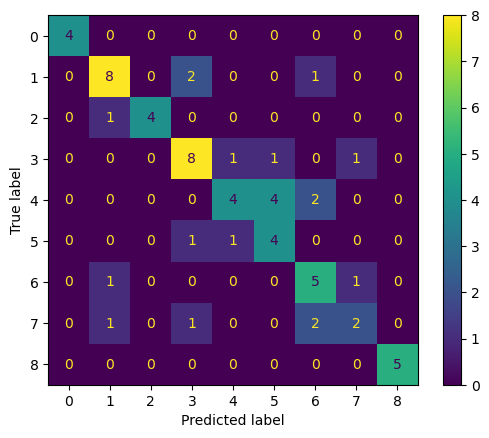
Accuracyprovides a general measure of how well the classifier performs overallIt is the Number of Correct Predictions divided by the Total Number of Samples
Precisionmeasures the proportion of true positive predictions relative to the total predicted positives for a classConfusion MatrixComputes the matrix summarizing the classifier’s predictions. Each row corresponds to the true label, and each column corresponds to the predicted label. The diagonal elements represent correctly classified samples, while off-diagonal elements represent misclassifications
# list the LandTypes and class
label_dfInterpret and Understand ML model
Model interpretation in machine learning is crucial for understanding how models make predictions, especially in complex models. SHAP (SHapley Additive exPlanations) scores are a popular method for interpreting model predictions. They provide a way to explain the output of any machine learning model by assigning each feature an importance value for a particular prediction.
SHAP scores explain the contribution of each feature to a model’s prediction using concepts from cooperative game theory. They start with a baseline prediction, which is the average prediction across all data points. For each feature, SHAP calculates how much the prediction changes when the feature is included compared to when it is not, considering all possible combinations of features. The SHAP value for a feature is the average of its contributions across all combinations, ensuring fair distribution.
Positive SHAP values indicate the feature increases the prediction, while negative values suggest it decreases it.
import shap
shap.initjs()

# Initialize the SHAP Tree Explainer for XGBoost
explainer = shap.TreeExplainer(best_model,feature_names=dsp.wavelength.values.astype(int).astype(str))
shap_values = explainer(X_test)Visualize a prediction’s explanation
Force Plot We can select an individual prediction to inspect how the input features have influenced its assignment to a class.
Features pushing the prediction higher are shown in red, those pushing the prediction lower are in blue
base value (the average model output over the training dataset we passed) to the model output
sel_in = 55

print(f"predicted class: {label_df.loc[y_pred[sel_in],'LandType']}")
print(f"true class: {label_df.loc[y_test[sel_in], 'LandType']}")
predicted class: Eucalyptus
true class: Eucalyptus
#lables for wavelength in plot
feats =  dsp.wavelength.values.astype(int).astype(str)
shap.force_plot(explainer.expected_value[y_test[sel_in]], shap_values.values[sel_in,:,y_test[sel_in]], pd.DataFrame(X_test).iloc[sel_in, :],link='logit',feature_names=list(feats))sel_in = 59
print(f"predicted class: {label_df.loc[y_pred[sel_in],'LandType']}")
print(f"true class: {label_df.loc[y_test[sel_in], 'LandType']}")predicted class: Forest
true class: Pine
#lables for wavelength in plot
feats =  dsp.wavelength.values.astype(int).astype(str)
shap.force_plot(explainer.expected_value[y_test[sel_in]], shap_values.values[sel_in,:,y_test[sel_in]], pd.DataFrame(X_test).iloc[sel_in, :],link='logit',feature_names=list(feats))Beeswarm We can also inspect the importance of features across all instances of a particular class.
To get an overview of which features are most important for a model we can plot the SHAP values of every feature for every sample
The color represents the feature value (red high, blue low)
sel_in = 55
shap.plots.beeswarm(shap_values[:,:,y_test[sel_in]])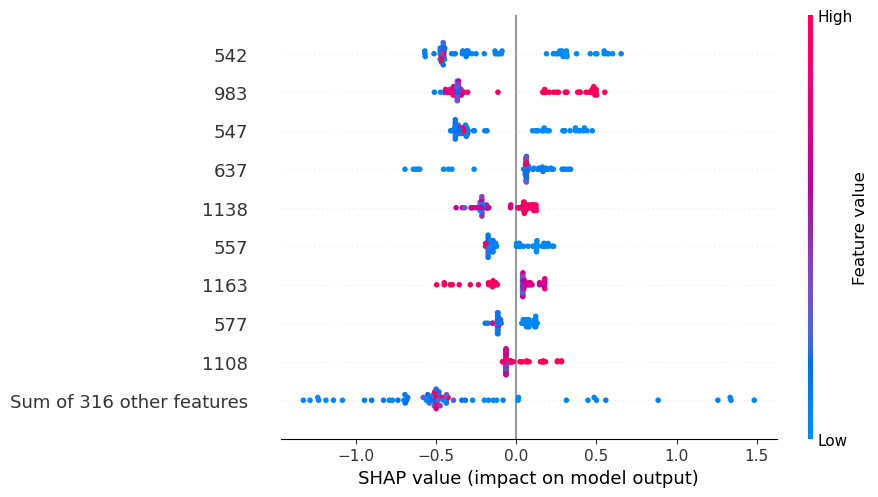
Finally, lets overlay this on the actual spectra for a individual observation to understand how spectral features are contributing to our predictions.
#plot spectra and importance
importance = np.abs(shap_values[sel_in,:,y_test[sel_in]].values)
# Create the base plot
fig, ax = plt.subplots(figsize=(12, 6))

# Get the wavelength and importance data
wavelength = dsp['wavelength'].values
importance = importance  # Make sure this aligns with your wavelength data

# Create a colormap
cmap = plt.get_cmap('hot').reversed()  # You can choose a different colormap if you prefer

# Normalize importance values to [0, 1] for colormap
norm = plt.Normalize(importance.min(), importance.max())

# Add shading
for i in range(len(wavelength) - 1):
    ax.fill_between([wavelength[i], wavelength[i+1]], 0, 1,
                    color=cmap(norm(importance[i])), alpha=0.3)

# Add a colorbar to show the importance scale
sm = plt.cm.ScalarMappable(cmap=cmap, norm=norm)
sm.set_array([])
cbar = plt.colorbar(sm, ax=ax, label='Importance')

# Add white blocks to obscure specified regions
ax.fill_between([0,450], 0, 1, color='white')
ax.fill_between([1340,1480], 0, 1, color='white')
ax.fill_between([1800,1980], 0, 1, color='white')
ax.fill_between([2400,2500], 0, 1, color='white')
ax.set_xlim(420,2400)

plot_xr = xr.DataArray(X_test[sel_in], coords=[wavelength], dims=["wavelength"])
plot_xr.plot.line(x='wavelength', color='green', ylim=(0, 0.2), ax=ax,zorder=0)

plt.title('Reflectance with Importance Shading')
plt.xlabel('Wavelength')
plt.ylabel('Reflectance (normalized)')

plt.tight_layout()
plt.show()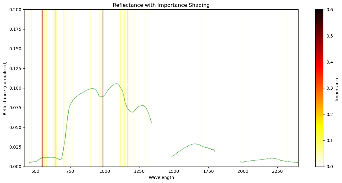
Deploy the Model to AVIRIS-NG Scenes
First, limit predictions to natural areas only
This model was only trained on data covering natural vegetaton in the Cape Peninsula, It is important that we only predict in the areas that match our training data. We will therefore filter to scenes that cover the Cape Peninsula and mask out non-protected areas.
#south africa protected areas
SAPAD = (gpd.read_file('data/SAPAD_2024.gpkg')
         .query("SITE_TYPE!='Marine Protected Area'")
        )
SAPAD.crs

SAPAD.keys()

m = SAPAD[['SITE_TYPE', 'geometry']].explore('SITE_TYPE')
mLimit the Cape Town Peninsula AVIRIS-NG scenes to those that intersect with the South Africa Protected Areas
#south africa protected areas
SAPAD = (gpd.read_file('data/SAPAD_2024.gpkg')
         .query("SITE_TYPE!='Marine Protected Area'")
        )
SAPAD = SAPAD.to_crs("EPSG:32734")

# Get the bounding box of the training data
bbox = class_data_utm.total_bounds  # (minx, miny, maxx, maxy)
gdf_bbox = gpd.GeoDataFrame({'geometry': [box(*bbox)]}, crs=class_data_utm.crs)  # Specify the CRS
gdf_bbox['geometry'] = gdf_bbox.buffer(500)

# protected areas that intersect with the training data
SAPAD_CT = SAPAD.overlay(gdf_bbox,how='intersection')

#keep only AVIRIS scenes that intersects with CT protected areas
AVNG_sapad = AVNG_CP[AVNG_CP.intersects(SAPAD_CT.unary_union)]

# plot
m = AVNG_sapad[['GranuleUR','geometry']].explore('GranuleUR')
mPredict over one AVIRIS scene
We now have a trained model and are ready to deploy it to generate predictions across an entire AVIRIS scene and map the distribution of invasive plants. This involves handling a large volume of data, so we need to write the code to do this intelligently. We will accomplish this by applying the .predict() method of our trained model in parallel across the chunks of the AVIRIS xarray. The model will receive one chunk at a time so that the data is not too large, but it will be able to perform this operation in parallel across multiple chunks, and therefore will not take too long.
Here is the function that we will actually apply to each chunk. Simple really. The hard work is getting the data into and out of this function
chunk- a portion of input data (e.g., a subset of the dataset) The function processes chunks for efficient computation and predictionmodel- This is our trained machine learning modelpredict_proba()is used to predict the class probabilities
def predict_on_chunk(chunk, model):
    probabilities = model.predict_proba(chunk)
    return probabilities
Now we define the function that takes as input the path to the AVIRIS file and pass the data to the predict function. This is composed of 4 parts:
Part 1: Opens the AVIRIS data file using xarray and sets a condition to identify valid data points where reflectance values are greater than zero.
Part 2: Applies all the transformations that need to be done before the data goes to the model. It puts the spatial dimensions (x and y) into a single dimension, filters wavelengths, and normalizes the reflectance data.
Part 3: Applies the machine learning model,
best_model, to the normalized data in parallel, predicting class probabilities for each data point using xarray’sapply_ufuncmethod. Most of the function involves defining what to do with the dimensions of the old dataset and the new outputPart 4: Unstacks the data to restore its original dimensions, sets spatial dimensions and coordinate reference system (CRS), clips the data, and transposes the data to match expected formats before returning the results.
def predict_xr(file,geometries):

    rfl_f, ql_f, unc_f = separate_granule_type(file)
    native_id = path.basename(rfl_f[0].path)[:-7]

    #part 1 - opening file
    #open the file
    print(f'file: {rfl_f[0]}')
    ds = xr.open_datatree(rfl_f[0], engine='h5netcdf', chunks='auto')

    #get the geometries of the protected areas for masking
    ds_crs = ds.transverse_mercator.crs_wkt
    geometries = geometries.to_crs(ds_crs).geometry.apply(mapping)

    #condition to use for masking no data later
    condition = (ds['reflectance'] > -1).any(dim='wavelength')

    #stack the data into a single dimension. This will be important for applying the model later
    ds = ds.reflectance.to_dataset().stack(sample=('easting','northing'))

    #part 2 - pre-processing
    #remove bad wavelenghts
    wavelengths_to_drop = ds.wavelength.where(
        (ds.wavelength < 450) |
        (ds.wavelength >= 1340) & (ds.wavelength <= 1480) |
        (ds.wavelength >= 1800) & (ds.wavelength <= 1980) |
        (ds.wavelength > 2400), drop=True
    )
    # Use drop_sel() to remove those specific wavelength ranges
    ds = ds.drop_sel(wavelength=wavelengths_to_drop)

    #normalise the AVIRIS data
    l2_norm = np.sqrt((ds['reflectance'] ** 2).sum(dim='wavelength'))
    ds['reflectance'] = ds['reflectance'] / l2_norm


    #part 3 - apply the model over chunks
    result = xr.apply_ufunc(
        predict_on_chunk,
        ds['reflectance'].chunk(dict(wavelength=-1)),
        input_core_dims=[['wavelength']],    # input dim with features
        output_core_dims=[['class']],        # name for the new output dim
        exclude_dims=set(('wavelength',)),   # dims to drop in result
        output_sizes={'class': 9},           # length of the new dimension
        output_dtypes=[np.float32],
        dask="parallelized",
        kwargs={'model': best_model}
    )

    #part 4 - post-processing
    result = result.where((result >= 0) & (result <= 1), np.nan)  # valid values
    result = result.unstack('sample')                             # remove the stack
    result = result.rio.set_spatial_dims(x_dim='easting',y_dim='northing') # set the spatial dims
    result = result.rio.write_crs(ds_crs)                         # set the CRS
    result = result.rio.clip(geometries)                          # clip to the protected areas and no data
    result = result.transpose('class', 'northing', 'easting')     # transpose the data - rio expects it this way

    return result
Let’s test that it works on a single file before we run it through 100s of GB of data.
test  = predict_xr(earthaccess.open(single_granule),SAPAD_CT)
testfile: <File-like object S3FileSystem, ornl-cumulus-prod-protected/bioscape/BioSCape_ANG_V02_L3_RFL_Mosaic/data/AVIRIS-NG_BIOSCAPE_V02_L3_36_11_RFL.nc>
The AVIRIS tile is AVIRIS-NG_BIOSCAPE_V02_L3_36_11_RFL.nc
# Again, recall the labels and LandType classes
label_dfLet’s plot an image of the tile’s AVIRIS-NG_BIOSCAPE_V02_L3_36_11_RFL.nc output. This takes some time to plot.
# Reproject the dataset to WGS84 (EPSG:4326)
test = test.rio.reproject("EPSG:4326", nodata=np.nan)

# Enhanced Plot with Titles and Styling
h = test.isel({'class': 6}).hvplot(
    tiles=hv.element.tiles.EsriImagery(),   # Use Esri Imagery as a tile background
    project=True,                          # Project the data to work seamlessly with the background
    rasterize=True,                        # Rasterize for efficient plotting
    clim=(0.01, 1),                           # Define color limits to focus on the range of interest
    cmap='turbo',                          # Colormap for better visualization
    frame_width=800,                       # Increase the width for better spatial resolution
    data_aspect=1,                         # Maintain a realistic and proportional aspect ratio
    alpha=0.5,                             # Adjust opacity for optimal visualization
    colorbar=True                          # Enable the colorbar (hvplot handles this properly)
)

# Add Descriptive Titles (handled internally by hvplot)
h = h.opts(
    title="Class6: Eucalyptus - Probability Mapping"  # Set title directly using Holoviews options
)
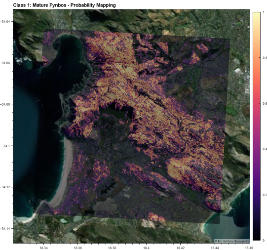
h ML models typically provide a single prediction of the most likely outcomes. You can also get probability-like scores (values from 0 to 1) from these models, but they are not true probabilities. If the model gives you a score of 0.6, that means it is more likely than a prediction of 0.5, and less likely than 0.7. However, it does not mean that in a large sample your prediction would be right 60 times out of 100. To get calibrated probabilities from our models, we have to apply additional steps. We can also get a set of predictions from models rather than a single prediction, which reflects the model’s true uncertainty using a technique called conformal predictions. Read more about conformal prediction for geospatial machine learning in this amazing paper:
OK, now we are ready to apply the prediction to each tile.
This loops through each AVIRIS-NG L3 tile, but won’t take long, as we have not yet asked it to perform the computation.
grid_pred = []
# loop over tile names intersecting the protected areas
for t in AVNG_sapad['GranuleUR'].to_list():
    # search for each tile
    g = earthaccess.search_data(
        doi='10.3334/ORNLDAAC/2427', # BioSCape: AVIRIS-NG L3
        granule_name = f"{t}*", # select the tile
    )
    # run prediction and append the output xarray to grid_pred
grid_pred.append(predict_xr(earthaccess.open(g),SAPAD_CT))file: <File-like object S3FileSystem, ornl-cumulus-prod-protected/bioscape/BioSCape_ANG_V02_L3_RFL_Mosaic/data/AVIRIS-NG_BIOSCAPE_V02_L3_37_11_RFL.nc>
file: <File-like object S3FileSystem, ornl-cumulus-prod-protected/bioscape/BioSCape_ANG_V02_L3_RFL_Mosaic/data/AVIRIS-NG_BIOSCAPE_V02_L3_37_12_RFL.nc>
file: <File-like object S3FileSystem, ornl-cumulus-prod-protected/bioscape/BioSCape_ANG_V02_L3_RFL_Mosaic/data/AVIRIS-NG_BIOSCAPE_V02_L3_34_12_RFL.nc>
file: <File-like object S3FileSystem, ornl-cumulus-prod-protected/bioscape/BioSCape_ANG_V02_L3_RFL_Mosaic/data/AVIRIS-NG_BIOSCAPE_V02_L3_38_11_RFL.nc>
file: <File-like object S3FileSystem, ornl-cumulus-prod-protected/bioscape/BioSCape_ANG_V02_L3_RFL_Mosaic/data/AVIRIS-NG_BIOSCAPE_V02_L3_36_10_RFL.nc>
file: <File-like object S3FileSystem, ornl-cumulus-prod-protected/bioscape/BioSCape_ANG_V02_L3_RFL_Mosaic/data/AVIRIS-NG_BIOSCAPE_V02_L3_35_10_RFL.nc>
file: <File-like object S3FileSystem, ornl-cumulus-prod-protected/bioscape/BioSCape_ANG_V02_L3_RFL_Mosaic/data/AVIRIS-NG_BIOSCAPE_V02_L3_37_10_RFL.nc>
file: <File-like object S3FileSystem, ornl-cumulus-prod-protected/bioscape/BioSCape_ANG_V02_L3_RFL_Mosaic/data/AVIRIS-NG_BIOSCAPE_V02_L3_36_12_RFL.nc>
file: <File-like object S3FileSystem, ornl-cumulus-prod-protected/bioscape/BioSCape_ANG_V02_L3_RFL_Mosaic/data/AVIRIS-NG_BIOSCAPE_V02_L3_39_12_RFL.nc>
file: <File-like object S3FileSystem, ornl-cumulus-prod-protected/bioscape/BioSCape_ANG_V02_L3_RFL_Mosaic/data/AVIRIS-NG_BIOSCAPE_V02_L3_38_12_RFL.nc>
file: <File-like object S3FileSystem, ornl-cumulus-prod-protected/bioscape/BioSCape_ANG_V02_L3_RFL_Mosaic/data/AVIRIS-NG_BIOSCAPE_V02_L3_36_11_RFL.nc>
file: <File-like object S3FileSystem, ornl-cumulus-prod-protected/bioscape/BioSCape_ANG_V02_L3_RFL_Mosaic/data/AVIRIS-NG_BIOSCAPE_V02_L3_34_11_RFL.nc>
file: <File-like object S3FileSystem, ornl-cumulus-prod-protected/bioscape/BioSCape_ANG_V02_L3_RFL_Mosaic/data/AVIRIS-NG_BIOSCAPE_V02_L3_35_12_RFL.nc>
Merge and Mosaic results
The results are now available as a list of xarrays, one for each scence. We want to combine these together into a single seamless mosaic for the entire Cape Peninsula. Fortunately we don’t have to write a ton of code to do this as rioxarray already has a mosaic function
from rioxarray.merge import merge_arraysThis next code block will force computation and take about 10-30 mins to run on a 4 core, 16GB RAM machine. We wont run this, but rather load the results computed earlier.
# merged = merge_arrays(grid_pred, nodata=np.nan)
# merged = merged.rio.reproject("EPSG:4326")
# merged.rio.to_raster('data/ct_invasive.tif',driver="COG")
Restart if/as Needed
The file we are about to load is large. If the kernel is restarted, we will remove all existing data and free up space. We will then need to reload packages.
import xarray as xr
import rioxarray as riox
import hvplot.xarray
import holoviews as hv
hvplot.extension('bokeh')
merged = xr.open_dataset('../../shared-public/BioSCape_AVIRIS-NG_L3/ct_invasive_2.tif', engine='rasterio', chunks='auto')
mergedview the result
h = merged.isel({'band':6}).hvplot(x='x',y='y',
                               tiles='ESRI',geo=True,
                                project=True,rasterize=True,
                                cmap='turbo',clim=(0,1), frame_width=400,data_aspect=1,alpha=0.5)
h = h.opts(
    title="Class6: Eucalyptus - Probability Mapping"  # Set title directly using Holoviews options
)
h
Now we can inspect our results. Where do they look good? Where do they look bad? We should at this point return to the beginning of our workflow and refine every step of the process. Probably most importantly we should update our training data to include points that correct the errors that we see in our earlier outputs. This process of using early predictions to update our data is called ‘Active Learning’
CREDITS:
Find all of the October 2025 BioSCape Data Workshop Materials/Notebooks
This Notebook is an adaption of Glenn Moncrieff’s BioSCape Data Workshop Notebook: Mapping invasive species using supervised machine learning and AVIRIS-NG
This Notebook accesses and uses an updated version of AVIRIS-NG data with improved corrections and that are in netCDF file formats
Glenn’s lesson borrowed from:
- Brodrick, P. G., Chlus, A. M., Eckert, R., Chapman, J. W., Eastwood, M., Geier, S., Helmlinger, M., Lundeen, S. R., Olson-Duvall, W., Pavlick, R., Rios, L. M., Thompson, D. R., & Green, R. O. (2025). BioSCape: AVIRIS-NG L3 Resampled Reflectance Mosaics, V2. Oak Ridge National Laboratory, Oak Ridge, Tennessee, USA. 10.3334/ORNLDAAC/2427