Summary
This notebook will demonstrate how to search, discover, subset, and access NASA airborne imaging spectrometer data derived from the AVIRIS (Airborne Visible / Infrared Imaging Spectrometers) suite of instruments. AVIRIS data are archived to NASA Earthdata collections, but but given the many years of flights in support of varied NASA campaigns, can be a challenge to discover and access.
The earthaccess Python library simplifies programmatic discovery and access of NASA Earthdata data including the many AVIRIS instrument’s radiance, reflectance, and further derived campaign data. earthaccess is a useful Python library that facilitates finding and downloading or streaming data over HTTPS or s3. earthaccess searches NASA’s Common Metadata Repository (CMR) which is a metadata system that catalogs Earth Science data and associated metadata records. This can then be used to download granules or generate lists of granule search result URLs.
With areas and times of interest identified, flight metadata will be used to build and visual flight paths within those subset parameters.
Background
Developed at the NASA Jet Propulsion Laboratory (JPL), the Airborne Visible / Infrared Imaging Spectrometers (AVIRIS) are a unique suite of optical sensors that collect data while mounted on airborne platforms such as the B200 LARC or an ER-2 AFRC. Imaging spectrometers collect light reflected off of an object (the Earth in this case) and then analyze the intensity of the wavelengths present at each pixel. As their names suggest, the AVIRIS instruments collect light in the visible to infrared wavelenths. These data can be used for characterization of the Earth’s surface and atmosphere and applied to studies in the fields of oceanography, environmental science, snow hydrology, geology, volcanology, soil and land management, atmospheric and aerosol studies, agriculture, and limnology.
Green, R.O., M.L. Eastwood, C.M. Sarture, T. G. Chrien, M. Aronsson, B.J. Chippendale, J.A. Faust, B.E. Pavri, C. J. Chovit, M. Solis, M.R. Olah, and O. Williams. 1998. Imaging Spectroscopy and the Airborne Visible/Infrared Imaging Spectrometer (AVIRIS). Remote Sensing of Environment 65:227- 248. Green et al. (1998)
Chadwick KD, Brodrick PG, Grant K, et al. Integrating airborne remote sensing and field campaigns for ecology and Earth system science. Methods Ecol Evol. 2020; 11: 1492–1508. Chadwick et al. (2020)
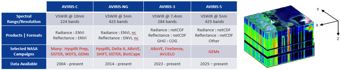
AVIRIS imaging spectrometers break down light into hundreds of narrow spectral bands, providing a spectrum for each point (or pixel) in the image. The resulting data are typically stored in a 3-dimensional array sometimes referred to as a data cube. The x and y dimensions represent the spatial dimensions of the image and the z dimension represents the wavelength information. JPL processes and provides data as radiance (L1B) and reflectance (L2A) which are archived and publically available through NASA Earthdata Facility Instrument Collections. These data files are historically distributed in a popular remote sensing ENVI file format and more recently as a standardized netCDF file format.
AVIRIS Data Processing Levels
| Level | Description |
|---|---|
| L1B | Resampled calibrated data in units of spectral radiance as well as observational geometry and illumination parameters |
| L2 | Calibrated Reflectance |
| L2A | Orthocorrected and atmospherically corrected reflectance data |
| L2B | Enhanced Surface Reflectance which can include topographic, glint, and bidirectional reflectance distribution function (BRDF) corrections |
| L3 | Variables are mapped on uniform space-time grid scales, usually with some completeness and consistency |
NASA Earthdata AVIRIS Project Data
Facility Instrument Links
AVIRIS-Classic: L1B Calibrated Radiance, Facility Instrument Collection, V1
AVIRIS-Classic: L2 Calibrated Reflectance, Facility Instrument Collection, V1
AVIRIS-NG L1B Calibrated Radiance, Facility Instrument Collection, V1
AVIRIS-NG L2 Surface Reflectance, Facility Instrument Collection, V1
AVIRIS-3 L1B Calibrated Radiance, Facility Instrument Collection
AVIRIS-3 L2A Orthocorrected Surface Reflectance, Facility Instrument Collection
Notebook Requirements
A NASA Earthdata Login account is required
Learning Objectives
login and authenticate to NASA Earthdata Login using earthaccess
construct searches of the NASA Common Metadata Repository (CMR) for specific airborne instruments
construct searches of the NASA Common Metadata Repository (CMR) for specific NASA Projects/Campaigns
narrow a search of the CMR to for files from AVIRIS instrument flights based on a spatial area of interest
programmatically discover specific AVIRIS- file access URLs based on metadata and spatial/temporal parameters
create flight line bounding boxes from a search result using CMR file(granule)-level metadata
Set Up
Import the required Python libraries
import earthaccess
import geopandas as gpd
import xarray as xr
import pandas as pd
from shapely.ops import orient
import warnings
# suppress future warnings
warnings.filterwarnings('ignore', category=FutureWarning)
earthaccess is a Python library that simplifies data discovery and access to NASA Earthdata data by providing an abstraction layer to NASA’s APIs for programmatic access.
earthaccess will be used to:
Authentication:- handles a user’s identity (authentication) with NASA’s Earthdata Login (EDL),Search:search the NASA Earthdata Data holdings using NASA’s Common Metadata Repository (CMR), andAccess:provide direct cloud file download and access
Earthdata Login
NASA Earthdata Login is a user registration and profile management system for users getting Earth science data from NASA Earthdata. If you download or access NASA Earthdata data, you need an Earthdata Login.
Authentication
Using earthaccess we’ll login and authenticate to NASA Systems.
For this exercise, we will be prompted for and interactively enter our Eathdata Login credentials (login, password)
auth = earthaccess.login()Searching by Collection
The earthaccess search_datasets function with the keyword argument can be used to search collections.
Given the many Instruments and Campaigns, there are several AVIRIS-* collections or datasets available within the NASA Earthdata cloud archive.
# Retrieve Collections
collections = earthaccess.search_datasets(keyword='AVIRIS')
# Print Quantity of Results
print(f'Collections found: {len(collections)}')
Collections found: 118
Printing the collections object explores all of the json metadata.
#Print collections
#printing the first index
collections[0]
{
"meta": {
"revision-id": 28,
"deleted": false,
"format": "application/vnd.nasa.cmr.umm+json",
"provider-id": "ORNL_CLOUD",
"has-combine": false,
"user-id": "jewellbc",
"has-formats": false,
"associations": {
"citations": [
"CIT3804235725-ESDIS",
"CIT4106707771-ESDIS"
]
},
"s3-links": [
"s3://ornl-cumulus-prod-protected/aviris/AVIRIS-Classic_L2_Reflectance/data",
"s3://ornl-cumulus-prod-public/aviris/AVIRIS-Classic_L2_Reflectance"
],
"has-spatial-subsetting": false,
"native-id": "AVIRIS-Classic_L2_Reflectance_2154",
"has-transforms": false,
"association-details": {
"citations": [
{
"concept-id": "CIT3804235725-ESDIS"
},
{
"concept-id": "CIT4106707771-ESDIS"
}
]
},
"has-variables": false,
"concept-id": "C2711871294-ORNL_CLOUD",
"revision-date": "2026-02-10T21:10:29.446Z",
"has-temporal-subsetting": false,
"concept-type": "collection"
},
"umm": {
"AncillaryKeywords": [
"calibrated surface reflectance",
"water absorption path",
"corrected surface reflectance"
],
"CollectionCitations": [
{
"OtherCitationDetails": "Green, R.O., D.R. Thompson, J.W. Boardman, J.W. Chapman, M. Eastwood, M. Helmlinger, S.R. Lundeen, and W. Olson-Duvall. 2023. AVIRIS-Classic: L2 Calibrated Reflectance, Facility Instrument Collection, V1. ORNL DAAC, Oak Ridge, Tennessee, USA. https://doi.org/10.3334/ORNLDAAC/2154"
}
],
"AdditionalAttributes": [
{
"Name": "FLIGHTLINE",
"Description": "Flightline",
"DataType": "STRING"
},
{
"Name": "Identifier_product_doi_authority",
"Description": "DOI Authority",
"DataType": "STRING"
},
{
"Name": "Campaign",
"Description": "Campaign",
"DataType": "STRING"
}
],
"SpatialExtent": {
"HorizontalSpatialDomain": {
"Geometry": {
"BoundingRectangles": [
{
"WestBoundingCoordinate": -171.842,
"NorthBoundingCoordinate": 48.6945,
"EastBoundingCoordinate": -81.0205,
"SouthBoundingCoordinate": 18.5747
}
],
"CoordinateSystem": "CARTESIAN"
}
},
"SpatialCoverageType": "HORIZONTAL",
"GranuleSpatialRepresentation": "CARTESIAN"
},
"CollectionProgress": "ACTIVE",
"StandardProduct": false,
"ScienceKeywords": [
{
"Category": "EARTH SCIENCE",
"Topic": "LAND SURFACE",
"Term": "SURFACE RADIATIVE PROPERTIES",
"VariableLevel1": "REFLECTANCE"
},
{
"Category": "EARTH SCIENCE",
"Topic": "ATMOSPHERE",
"Term": "ATMOSPHERIC WATER VAPOR",
"VariableLevel1": "WATER VAPOR INDICATORS",
"VariableLevel2": "WATER VAPOR"
}
],
"TemporalExtents": [
{
"RangeDateTimes": [
{
"BeginningDateTime": "2008-06-11T00:00:00.000Z"
}
],
"EndsAtPresentFlag": true
}
],
"ProcessingLevel": {
"ProcessingLevelDescription": "Derived geophysical variables at the same resolution as L1 source data",
"Id": "2"
},
"DOI": {
"DOI": "10.3334/ORNLDAAC/2154",
"Authority": "https://doi.org"
},
"ShortName": "AVIRIS-Classic_L2_Reflectance_2154",
"EntryTitle": "AVIRIS-Classic: L2 Calibrated Reflectance, Facility Instrument Collection, V1",
"DirectDistributionInformation": {
"Region": "us-west-2",
"S3BucketAndObjectPrefixNames": [
"s3://ornl-cumulus-prod-protected/aviris/AVIRIS-Classic_L2_Reflectance/data",
"s3://ornl-cumulus-prod-public/aviris/AVIRIS-Classic_L2_Reflectance"
],
"S3CredentialsAPIEndpoint": "https://data.ornldaac.earthdata.nasa.gov/s3credentials",
"S3CredentialsAPIDocumentationURL": "https://data.ornldaac.earthdata.nasa.gov/s3credentialsREADME"
},
"RelatedUrls": [
{
"Description": "Earthdata Search allows users to search, discover, visualize, refine, and access NASA Earth Observation data.",
"URLContentType": "DistributionURL",
"Type": "GET DATA",
"Subtype": "Earthdata Search",
"URL": "https://search.earthdata.nasa.gov/search?q=AVIRIS-Classic_L2_Reflectance_2154&ac=true"
},
{
"Description": "Data set Landing Page DOI URL",
"URLContentType": "CollectionURL",
"Type": "DATA SET LANDING PAGE",
"URL": "https://doi.org/10.3334/ORNLDAAC/2154"
},
{
"Description": "Browse Image",
"URLContentType": "VisualizationURL",
"Type": "GET RELATED VISUALIZATION",
"URL": "https://daac.ornl.gov/AVIRIS/guides/AVIRIS-Classic_L2_Reflectance_Fig1.jpg"
},
{
"Description": "ORNL DAAC Data Set Documentation",
"URLContentType": "PublicationURL",
"Type": "VIEW RELATED INFORMATION",
"Subtype": "USER'S GUIDE",
"URL": "https://data.ornldaac.earthdata.nasa.gov/public/aviris/AVIRIS-Classic_L2_Reflectance/comp/AVIRIS-Classic_L2_Reflectance.pdf"
},
{
"Description": "AVIRIS-Classic: L2 Calibrated Reflectance, Facility Instrument Collection, V1: AVIRIS-Classic_L2_Reflectance.pdf",
"URLContentType": "PublicationURL",
"Type": "VIEW RELATED INFORMATION",
"Subtype": "GENERAL DOCUMENTATION",
"URL": "https://data.ornldaac.earthdata.nasa.gov/public/aviris/AVIRIS-Classic_L2_Reflectance/comp/AVIRIS-Classic_L2_Reflectance.pdf"
}
],
"DataDates": [
{
"Date": "2023-06-15T11:48:39.000Z",
"Type": "CREATE"
},
{
"Date": "2025-11-21T10:49:52.000Z",
"Type": "UPDATE"
}
],
"Abstract": "This dataset contains Level 2 (L2) orthocorrected reflectance from the Airborne Visible / Infrared Imaging Spectrometer (AVIRIS-Classic) instrument. This is the NASA Earth Observing System Data and Information System (EOSDIS) facility instrument archive of these data. The NASA AVIRIS-Classic is a pushbroom spectral mapping system with high signal-to-noise ratio (SNR), designed and toleranced for high performance spectroscopy. AVIRIS-Classic measures reflected radiance in 224 contiguous bands at approximately 10-nm intervals in the Visible to Shortwave Infrared (VSWIR) spectral range from 400-2500 nm. The AVIRIS-Classic sensor has a 1 milliradian instantaneous field of view, providing altitude dependent ground sampling distances from 20 m to sub meter range. AVIRIS-Classic is flown on a variety of aircraft platforms including the Twin Otter, NASA's WB-57, and NASA's high altitude ER-2. For each flight line, two types of L2 data files may be included: (a) calibrated surface reflectance and (b) water vapor and optical absorption paths for liquid water and ice. The L2 data are provided in ENVI format, which includes a flat binary file accompanied by a header (.hdr) file holding metadata in text format. This archive currently includes data from 2008 - 2025. Additional AVIRIS-Classic facility instrument L2 data will be added as they become available. AVIRIS-Classic supports NASA Science and applications in many areas including plant composition and function, geology and soils, greenhouse gas mapping, and calibration of orbital platforms.",
"LocationKeywords": [
{
"Category": "CONTINENT",
"Type": "NORTH AMERICA",
"Subregion1": "CANADA"
},
{
"Category": "CONTINENT",
"Type": "NORTH AMERICA",
"Subregion1": "UNITED STATES OF AMERICA"
},
{
"Category": "CONTINENT",
"Type": "NORTH AMERICA",
"Subregion1": "MEXICO"
},
{
"Category": "CONTINENT",
"Type": "NORTH AMERICA",
"Subregion1": "UNITED STATES OF AMERICA",
"Subregion2": "HAWAII"
},
{
"Category": "OCEAN",
"Type": "PACIFIC OCEAN",
"Subregion1": "EASTERN PACIFIC OCEAN"
}
],
"Version": "1",
"Projects": [
{
"ShortName": "AVIRIS",
"LongName": "Airborne Visible InfraRed Imaging Spectrometer"
}
],
"UseConstraints": {
"LicenseURL": {
"Linkage": "https://science.nasa.gov/earth-science/earth-science-data/data-information-policy",
"Name": "Data Use Policy",
"Description": "License URL for data use policy",
"MimeType": "text/html"
}
},
"DataCenters": [
{
"Roles": [
"ARCHIVER"
],
"ContactInformation": {
"ContactMechanisms": [
{
"Type": "Direct Line",
"Value": "(865) 241-3952"
},
{
"Type": "Email",
"Value": "uso@daac.ornl.gov"
}
],
"Addresses": [
{
"StreetAddresses": [
"ORNL DAAC User Services Office, P.O. Box 2008, MS 6407, Oak Ridge National Laboratory"
],
"City": "Oak Ridge",
"StateProvince": "Tennessee",
"Country": "USA",
"PostalCode": "37831-6407"
}
]
},
"ShortName": "ORNL_DAAC",
"LongName": "THE OAK RIDGE NATIONAL LABORATORY (ORNL) DISTRIBUTED ACTIVE ARCHIVE CENTER (DAAC)"
}
],
"Platforms": [
{
"ShortName": "NOAA Twin Otter",
"Type": "Propeller",
"LongName": "NOAA De Havilland DHC-6-300 Twin Otter",
"Instruments": [
{
"ShortName": "AVIRIS",
"LongName": "Airborne Visible InfraRed Imaging Spectrometer"
}
]
},
{
"ShortName": "NASA ER-2",
"Type": "Jet",
"LongName": "NASA Earth Resources-2",
"Instruments": [
{
"ShortName": "AVIRIS",
"LongName": "Airborne Visible InfraRed Imaging Spectrometer"
}
]
},
{
"ShortName": "NASA WB-57F",
"Type": "Jet",
"Instruments": [
{
"ShortName": "AVIRIS",
"LongName": "Airborne Visible InfraRed Imaging Spectrometer"
}
]
}
],
"MetadataSpecification": {
"URL": "https://cdn.earthdata.nasa.gov/umm/collection/v1.18.5",
"Name": "UMM-C",
"Version": "1.18.5"
},
"ArchiveAndDistributionInformation": {
"FileDistributionInformation": [
{
"Format": "multiple",
"TotalCollectionFileSize": 23.971,
"TotalCollectionFileSizeUnit": "TB"
}
]
}
}
}We can create a list of the short-name, concept-id, version, and EntryTitle of each result collection using list comprehension. These fields are important for specifying and searching for data within collections.
collections_info = [
    {
        'short_name': c.get_umm("ShortName"),
        'collection_concept_id': c["meta"]["concept-id"],
        'version': c.get_umm('Version'),
        'entry_title': c.get_umm('EntryTitle')
    }
    for c in collections
]
pd.set_option('display.max_colwidth', 150)
collections_info = pd.DataFrame(collections_info)
collections_infoSearching by Instrument
#instrument = earthaccess.search_datasets(instrument="AVIRIS-3")
instrument = earthaccess.search_datasets(instrument="AVIRIS-NG")
#instrument = earthaccess.search_datasets(instrument="AVIRIS") # AVIRIS-Classic
print(f"Total Datasets (instrument) found: {len(instrument)}")
Total Datasets (instrument) found: 35
instrument_info = [
    {
        'short_name': i.get_umm("ShortName"),
        'collection_concept_id': i["meta"]["concept-id"],
        'version': i.get_umm('Version'),
        'entry_title': i.get_umm('EntryTitle')
    }
    for i in instrument
]
pd.set_option('display.max_colwidth', 150)
instrument_info = pd.DataFrame(instrument_info)
instrument_infoThe collection concept-id or short_name are unique to each collection. After finding the collection you want to search, you can use the short_name or concept-id to search for granules (or files) within that collection.
Searching by Project
results = earthaccess.search_datasets(project="BioSCape")
#results = earthaccess.search_datasets(project="ABoVE")
print(f"Total Datasets (results_projects) found: {len(results)}")
Total Datasets (results_projects) found: 11
for item in results:
    print(item.get_umm("ShortName"))
BioSCape_EstuaryVegHabitats_2441
BioSCape_VegPlots_Berg_Eerste_2425
BioSCape_AVNG_L2B_BRDF_GCFR_2385
BioSCape_ANG_V02_L3_RFL_Mosaic_2427
Acoustic_Data_Cape_Floristic_2372
BioSCape_PRISM_L1B_RDN_2493
BioSCape_PRISM_L2A_RFL_2494
BioSCape_foliar_trait_spec_2482
LVISF1B
LVISF2
OLVIS1A
Search AVIRIS-3 Instrument (only) for Specific Project/Campaign
AVIRIS-3 datasets contain
campaigninformation at the granule level within the Unified Metadata Model-Granule (UMM-G)AdditionalAttributesFor AVIRIS-3 L1B data, this next code block lists the campaigns and number of granules in each campaign
Note that at the time of writing this Notebook, this functionality is specific to AVIRIS-3 Datasets
def  get_campaign_names(granules):
    """get campaign names for all granules"""
    c = []
    for g in granules:
        for attrs in g["umm"]['AdditionalAttributes']:
            if attrs['Name'] == 'Campaign':
                c += attrs['Values']
    return c

# earthdata search
granules = earthaccess.search_data(
    short_name = 'AV3_L1B_RDN_2356',
    #doi="10.3334/ORNLDAAC/2356"
)

campaigns = get_campaign_names(granules)

#print campaign names and granules
for name in list(set(campaigns)):
    print(f'{name} --> {campaigns.count(name)} granules')
MAGEQ --> 3225 granules
2025 LA Fires --> 292 granules
Calibration / Validation / Instrument Science / Testing --> 744 granules
DEVELOP Santa Clarita Valley Ecological Conservation --> 28 granules
SHIFT --> 55 granules
SCOAPE-II --> 625 granules
Carbon Mapper --> 4469 granules
AVUELO --> 1652 granules
GHG --> 1670 granules
AiRMAPS --> 2572 granules
GEMx --> 39 granules
NEON --> 16 granules
WDTS --> 507 granules
ABoVE --> 1405 granules
PACE --> 120 granules
AVIRIS4Acres --> 792 granules
FireSense --> 1838 granules
Sacramento Delta --> 1507 granules
If you know a NASA Project or Campaign employed the AVIRIS-3 instrument, you can directly query the AdditionalAttributes
#doi="10.3334/ORNLDAAC/2356" # AV3_L1B_RDN_2356
short_name = "AV3_L1B_RDN_2356"
query = earthaccess.DataGranules().short_name(short_name)
query.params['attribute[]'] = 'string,Campaign,SHIFT'
l1b = query.get_all()
print(f'Granules found: {len(l1b)}')
Granules found: 55
Setting Search Parameters for Granules
We’ll use a NEON AOP Flight Boundary to search for AVIRIS data in a spatial area of interest.
# read the AVIRIS-NG_flights.shp file and convert to geojson using geopandas
AOP_polys = gpd.read_file('data/AOP_flightboxesAllSites.shp')
AOP_polys.to_file('aop_json.geojson', driver='GeoJSON')
gdf = gpd.read_file('aop_json.geojson')
# Access the CRS using the .crs attribute
if gdf.crs:
print(f"CRS: {gdf.crs}")CRS: EPSG:4326
gdf.explore()serc_aop = gdf[(gdf['siteID'] == 'SJER') & (gdf['priority'] == 1)]
#serc_aop = gdf[(gdf['siteID'] == 'BARR') & (gdf['priority'] == 1)]print(serc_aop.head()) domain domainName siteName siteID \
60 D17 Pacific Southwest San Joaquin Experimental Range NEON SJER
siteType sampleType priority version flightbxID \
60 Core Terrestrial 1 2 D17_SJER_C1_P1_v2
geometry
60 POLYGON ((-119.78852 37.04531, -119.78852 37.13542, -119.67604 37.13542, -119.67604 37.04531, -119.78852 37.04531))
serc_aop.explore()Use the NEON AOP Boundary file to search for AVIRIS-Classic L2 Reflectance data within that boundary
# bounding lon, lat as a list of tuples
bounds = serc_aop.geometry.apply(orient, args=(1,))
bounds
# simplifying the polygon to bypass the coordinates
# limit of the CMR with a tolerance of .01 degrees
xy = bounds.simplify(0.01).get_coordinates()
print(xy)

date_range = ("2019-01-01", "2019-12-31")

results = earthaccess.search_data(
    short_name = 'AVIRIS-Classic_L2_Reflectance_2154',
    #short_name = 'ABoVE_Airborne_AVIRIS_NG_V3_2362',
    #short_name = 'AVIRIS-NG_L2_Reflectance_2110	',
    #short_name = 'AVIRIS-NG_L1B_radiance_2095',
    polygon=list(zip(xy.x, xy.y)),
    temporal = date_range
)
print(f"Total AVIRIS collections found: {len(results)}")
x y
60 -119.788522 37.045310
60 -119.676038 37.045310
60 -119.676038 37.135416
60 -119.788522 37.135416
60 -119.788522 37.045310
Total AVIRIS collections found: 3
For our search parameters, let’s explore the granules found
Let’s look at the first result
results[:1][Collection: {'ShortName': 'AVIRIS-Classic_L2_Reflectance_2154', 'Version': '1'}
Spatial coverage: {'HorizontalSpatialDomain': {'Geometry': {'GPolygons': [{'Boundary': {'Points': [{'Longitude': -119.7805, 'Latitude': 36.6489}, {'Longitude': -119.5878, 'Latitude': 36.6533}, {'Longitude': -119.6413, 'Latitude': 38.191}, {'Longitude': -119.838, 'Latitude': 38.1864}, {'Longitude': -119.7805, 'Latitude': 36.6489}]}}]}}}
Temporal coverage: {'RangeDateTime': {'BeginningDateTime': '2019-10-01T18:01:00Z', 'EndingDateTime': '2019-10-01T18:51:00Z'}}
Size(MB): 11973.347121238708
Data: ['https://data.ornldaac.earthdata.nasa.gov/protected/aviris/AVIRIS-Classic_L2_Reflectance/data/f191001t01p00r06_h2o_v1l1_img.bin', 'https://data.ornldaac.earthdata.nasa.gov/protected/aviris/AVIRIS-Classic_L2_Reflectance/data/f191001t01p00r06_h2o_v1l1_img.hdr', 'https://data.ornldaac.earthdata.nasa.gov/protected/aviris/AVIRIS-Classic_L2_Reflectance/data/f191001t01p00r06_corr_v1l1_img.hdr', 'https://data.ornldaac.earthdata.nasa.gov/protected/aviris/AVIRIS-Classic_L2_Reflectance/data/f191001t01p00r06_corr_v1l1_img.bin']]results[0]You can download these files directly to your local machine by clicking on any of the files
We also see that these data are Cloud Hosted: True
Create and Visualize the Bounding Boxes of the subset of files
From each granule, we’ll use the CMR Geometry information to create a plot of the AVIRIS-3 flight lines from our temporal and spatial subset
Below, we convert NASA’s Unified Metadata Model (UMM) geometry to a geopandas dataframe to plot the search results over a basemap.
subset_gdf = gpd.GeoDataFrame(results, geometry=gpd.GeoSeries(results, crs=4326))
subset_gdf.crs
<Geographic 2D CRS: EPSG:4326>
Name: WGS 84
Axis Info [ellipsoidal]:
- Lat[north]: Geodetic latitude (degree)
- Lon[east]: Geodetic longitude (degree)
Area of Use:
- name: World.
- bounds: (-180.0, -90.0, 180.0, 90.0)
Datum: World Geodetic System 1984 ensemble
- Ellipsoid: WGS 84
- Prime Meridian: Greenwichsubset_gdf.explore(fill=False, tiles='https://mt1.google.com/vt/lyrs=s&x={x}&y={y}&z={z}', attr='Google')# Create the base map with `serc_aop`
base_map = serc_aop.explore(
color="red", # Outline color for serc_aop features
fill=False, # No fill for serc_aop
legend=True, # Display legend for serc_aop
tiles='https://mt1.google.com/vt/lyrs=s&x={x}&y={y}&z={z}', # Google Satellite tiles
attr='Google'
)
# Add `subset_gdf` layer to the base map
final_map = subset_gdf.explore(
color="blue", # Outline color for subset_gdf features
fill=False, # No fill for subset_gdf
legend=True, # Display legend for subset_gdf
m=base_map # Add this layer to the base map
)
# Display the map
final_map- Green, R. O., Eastwood, M. L., Sarture, C. M., Chrien, T. G., Aronsson, M., Chippendale, B. J., Faust, J. A., Pavri, B. E., Chovit, C. J., Solis, M., Olah, M. R., & Williams, O. (1998). Imaging Spectroscopy and the Airborne Visible/Infrared Imaging Spectrometer (AVIRIS). Remote Sensing of Environment, 65(3), 227–248. 10.1016/s0034-4257(98)00064-9
- Chadwick, K. D., Brodrick, P. G., Grant, K., Goulden, T., Henderson, A., Falco, N., Wainwright, H., Williams, K. H., Bill, M., Breckheimer, I., Brodie, E. L., Steltzer, H., Williams, C. F. R., Blonder, B., Chen, J., Dafflon, B., Damerow, J., Hancher, M., Khurram, A., … Maher, K. (2020). Integrating airborne remote sensing and field campaigns for ecology and Earth system science. Methods in Ecology and Evolution, 11(11), 1492–1508. 10.1111/2041-210x.13463