Overview
The Portable Remote Imaging SpectroMeter (PRISM) is a compact airborne pushbroom imaging spectrometer built by the NASA Jet Propulsion Laboratory (JPL) for studies of coastal and inland waters. PRISM instrument covers spectral range from 350–1050 nm with with a 2.83 nm sampling per pixel, and a 0.88 mrad instantaneous field of view, with 608 cross-track pixels in a pushbroom configuration (Mouroulis et al., 2014).
In September 2024, PRISM flew on the NASA ER-2 high-altitude aircraft for the Plankton, Aerosol, Cloud, ocean Ecosystem Postlaunch Airborne eXperiment (PACE-PAX). PACE-PAX was a field campaign over Southern and Central California and adjacent coastal waters that collected validation data for the NASA PACE satellite and the JAXA/ESA EarthCARE satellite. The NASA ER-2 flew 13 research flights with six instruments that act as airborne proxies for the satellite sensors. PRISM covers lower-reflectance spectra for ocean colors, while PICARD has VNIR to SWIR channels. PRISM, together with the PICARD imaging spectrometer, matches capabilities of the PACE Ocean Color Instrument (OCI) (Knobelspiesse et al., 2026). The campaign sampled ocean color, aerosols, and clouds, including wildfire smoke over the Los Angeles region and red tide events in Monterey Bay.
In this tutorial, we use earthaccess to discover and download PRISM Level 1B (L1B) calibrated radiance for PACE-PAX. We then use a geometric lookup table (GLT) to orthorectify the image, and compare radiance spectra of water, sand, vegetation, and urban surfaces over Monterey Bay, California. We will also find the PACE OCI surface reflectance for the same surfaces.
Dataset
| Dataset | DOI | Short Name |
|---|---|---|
| PRISM: L1B Calibrated Radiance for PACE-PAX, 2024 | Bender et al. (2026) | PRISM_L1B_PACEPAX_2024_2515 |
| PACE OCI Level-2 Regional Surface Reflectance, version 3.1 | NASA Ocean Biology Processing Group (2025) | PACE_OCI_L2_SFREFL |
Learning Objectives
Search the PRISM PACE-PAX collection and its granules with
earthaccessStream a granule and explore its data structure
Orthorectify a calibrated radiance using the geometric lookup table (GLT)
Export an orthorectified image as a Cloud Optimized GeoTIFF
Find the PACE OCI surface reflectance for the same locations
Prerequisites
A free NASA Earthdata Login account is required. See the prerequisites page for setup instructions.
Import Libraries
import earthaccess
import numpy as np
import pandas as pd
import geopandas as gpd
import xarray as xr
import rioxarray
import pyproj
import matplotlib.pyplot as plt
import cartopy.crs as ccrs
import cartopy.io.img_tiles as cimgt
import warnings
warnings.filterwarnings('ignore')

xyz = "https://server.arcgisonline.com/ArcGIS/rest/services/World_Imagery/MapServer/tile/{z}/{y}/{x}"
attr = "ESRI"Authentication
Use earthaccess.login() to authenticate with your NASA Earthdata Login credentials. If you have a .netrc file configured, login will complete without a prompt.
auth = earthaccess.login()Search for the PRISM Collection
We search for the datasets from the PRISM instrument using earthaccess.
instrument = "PRISM"
datasets = earthaccess.search_datasets(instrument=instrument)
print(f"{instrument} datasets found: {len(datasets)}\n")
for ds in datasets:
    print(f"  Short name : {ds['umm']['ShortName']}")
PRISM datasets found: 28
Short name : ALOS_PRISM_L1B
Short name : BioSCape_PRISM_L1B_RDN_2493
Short name : BioSCape_PRISM_L2A_RFL_2494
Short name : CEOS_CalVal_Test_Site-Dome_C-Antarctica
Short name : CEOS_CalVal_Test_Site-Dunhuang-China
Short name : CEOS_CalVal_Test_Site-Frenchman_Flat-USA
Short name : CEOS_CalVal_Test_Site-Ivanpah_Playa-USA
Short name : CEOS_CalVal_Test_Site-La_Crau-France
Short name : CEOS_CalVal_Test_Site-Libya1
Short name : CEOS_CalVal_Test_Site-Libya4
Short name : CEOS_CalVal_Test_Site-Mauritania1
Short name : CEOS_CalVal_Test_Site-Negev-Southern_Israel
Short name : CEOS_CalVal_Test_Site-Railroad_Valley_Playa-USA
Short name : CEOS_CalVal_Test_Site-Tuz_Golu-Turkey
Short name : CEOS_CalVal_Test_Sites-Algeria3
Short name : CEOS_CalVal_Test_Sites-Algeria5
Short name : CEOS_CalVal_Test_Sites-Mauritania2
Short name : CNDP_CNDP_20240203_GEOCHEM_DATA
Short name : PACE-PAX_AircraftRemoteSensing_ER2_PRISM-PICARD-L1C_Data
Short name : PRISM_CORAL_L1
Short name : PRISM_CORAL_L2
Short name : PRISM_L1B_PACEPAX_2024_2515
Short name : SMODE_L1_PRISM_V1
Short name : SMODE_L2_PRISM_CHLA_V1
Short name : SMODE_L2a_PRISM_REFL_V1
Short name : USGS_BRD_NIISS
Short name : alos-prism-l1c
Short name : alos.prism.l1c.european.coverage.cloud.free
There are many datasets from the PRISM instruments published on NASA Earthdata. We will use PRISM_L1B_PACEPAX_2024_2515 dataset and print key metadata.
shortname = "PRISM_L1B_PACEPAX_2024_2515"
collections = earthaccess.search_datasets(short_name=shortname)

for c in collections:
    temporal = c.get_umm('TemporalExtents')[0]['RangeDateTimes'][0]
    print(f"Title      : {c.get_umm('EntryTitle')}")
    print(f"ShortName  : {c.get_umm('ShortName')}")
    print(f"Temporal   : {temporal['BeginningDateTime']} to {temporal['EndingDateTime']}")
    size = c.get_umm('ArchiveAndDistributionInformation')['FileDistributionInformation'][0]
    print(f"Total size : {size['TotalCollectionFileSize']} {size['TotalCollectionFileSizeUnit']}")
Title : PRISM: L1B Calibrated Radiance for PACE-PAX, 2024
ShortName : PRISM_L1B_PACEPAX_2024_2515
Temporal : 2024-09-04T00:00:00.000Z to 2024-09-30T23:59:59.999Z
Total size : 1.252 TB
Search for Granules
Each granule is one scene from a PRISM flight line. The file names follow the convention:
PACEPAX-PRISM-L1B_ER2_<YYYYMMDDhhmmss>_R0_<scene>.nc
where <YYYYMMDDhhmmss> is the start time of the flight line (UTC), R0 is the processing revision, and <scene> is the three-digit scene number within the flight line. We search for all granules in the collection and parse the flight line and scene from each file name. The dataset contains 2,223 NetCDF-4 files, each about 600 MB in size. Please refer to the user guide for full dataset documentation.
short_name = 'PRISM_L1B_PACEPAX_2024_2515'
granules = earthaccess.search_data(short_name=short_name)
print(f"Granules found: {len(granules)}")
Granules found: 2223
Let’s split the granule names into flight and scene.
def granule_details(g):
    gname = g.data_links()[0].split('/')[-1]
    sp = gname.removesuffix('.nc').split('_')
    return {
        'file': gname,
        'flight_line': sp[2],
        'scene': sp[-1],
        'start_time': pd.to_datetime(g['umm']['TemporalExtent']['RangeDateTime']['BeginningDateTime']),
        'size_mb': g['size'],
    }

df_granules = pd.DataFrame([granule_details(g) for g in granules])
df_granules.head()We summarize the scenes by flight day. PRISM collected data for several flight days between 4 and 30 September 2024.
df_granules['date'] = df_granules['start_time'].dt.date
df_granules.groupby('date').agg(
    flight_lines=('flight_line', 'nunique'),
    scenes=('file', 'count'),
    size_gb=('size_mb', lambda s: round(s.sum() / 1000, 1)),
)Find granules over Monterey Bay
Monterey Bay was a key PACE-PAX ocean target. A red tide was observed during the campaign (Knobelspiesse et al., 2026).
We search for granules that intersect a bounding box over Monterey bay and map their footprints.
# bounding box (west, south, east, north) over Monterey Bay, California
bbox = (-122.2, 36.5, -121.75, 37.05)

granules_mb = earthaccess.search_data(short_name=short_name,
                                      bounding_box=bbox)
print(f"Granules over Monterey Bay: {len(granules_mb)}")
Granules over Monterey Bay: 55
Let’s convert the granules to a geopandas dataframe and print summary details.
# convert to geopandas
gdf = gpd.GeoDataFrame(
    [granule_details(g) for g in granules_mb],
    geometry=gpd.GeoSeries(granules_mb, crs=4326),
)
gdf['start_time'] = gdf['start_time'].astype(str)
gdf.groupby('flight_line').size().rename('scenes').to_frame()# plot granule footprints, colored by flight line
gdf.explore(
column='flight_line', tiles=xyz, attr=attr, cmap='tab10',
style_kwds={"weight": 2, "fillOpacity": 0.5},
tooltip=['file', 'start_time'],
)Preview a granule
Each granule has an associated quick-look browse image, which can be used to scan the scene for any cloud cover and pick a clear scene. One of the clear scene is flight line 20240926181605, scene 019, acquired on 26 September 2024 over the area.
granule_name = 'PACEPAX-PRISM-L1B_ER2_20240926181605_R0_019.nc'
granule = [g for g in granules_mb if g.data_links()[0].endswith(granule_name)][0]

granuleOpen a Granule
We open and stream the granule with earthaccess.open().
f = earthaccess.open([granule])[0]
print(f"Granule opened: {f}")Granule opened: <File-like object S3FileSystem, ornl-cumulus-prod-protected/prism/PRISM_L1B_PACEPAX_2024/data/PACEPAX-PRISM-L1B_ER2_20240926181605_R0_019.nc>
Explore the NetCDF File Structure
PRISM L1B files are NetCDF-4 files with groups. We open the whole file as an xarray.DataTree to see all groups at once.
dt = xr.open_datatree(f, engine='h5netcdf')
dtThe file has three parts:
| Group | Variables | Description |
|---|---|---|
/ (root) | lat, lon, elev | Latitude, longitude, and surface elevation for each pixel in the raw (sensor) geometry, with dimensions (lines, samples). |
/radiance | radiance, wavelength, fwhm | Calibrated at-sensor radiance (µW nm⁻¹ cm⁻² sr⁻¹) with dimensions (wavelength, lines, samples), plus band center wavelengths and full width at half maximum (FWHM). |
/geolocation_lookup_table | line, sample, easting, northing | The geometric lookup table (GLT): a north-up UTM grid where each cell stores the raw line and sample of the pixel that belongs there. |
The radiance is in the raw geometry of the pushbroom sensor, which is not orthorectified. lines is the along-track direction (flight direction) and samples is the across-track direction. The nodata value is -9999; xarray masks it as NaN automatically.
We extract each group as an xarray.Dataset.
root = dt.to_dataset()
rad = dt['radiance'].to_dataset()
glt = dt['geolocation_lookup_table'].to_dataset()

print(dt.attrs['title'])
print(f"Acquisition: {dt.attrs['time_coverage_start']} to {dt.attrs['time_coverage_end']}")
print(f"Radiance shape (wavelength, lines, samples): {rad['radiance'].shape}")
print(f"GLT shape (northing, easting): {glt['line'].shape}")
PRISM L1B Calibrated Radiance (flight line: prm20240926t181605, scene: 019)
Acquisition: 2024-09-26T18:33:26Z to 2024-09-26T18:34:20Z
Radiance shape (wavelength, lines, samples): (246, 640, 606)
GLT shape (northing, easting): (672, 652)
The UTM zone of the GLT differs between flight lines (from UTM zones 9N to 12N in this dataset). The coordinate reference system (CRS) is stored in the transverse_mercator variable.
crs = pyproj.CRS.from_wkt(dt['transverse_mercator'].attrs['crs_wkt'])
pixel_size = float(glt['easting'].diff('easting')[0])
print(f"CRS: {crs.name} (EPSG:{crs.to_epsg()})")
print(f"GLT pixel size: {pixel_size:.1f} m")
CRS: WGS 84 / UTM zone 10N (EPSG:32610)
GLT pixel size: 17.9 m
Spectral Characteristics
PRISM measures 246 contiguous spectral bands, with following details.
wl = rad['wavelength']
fwhm = rad['fwhm']
print(f"Number of bands : {wl.size}")
print(f"Wavelength range : {wl.min():.1f} to {wl.max():.1f} nm")
print(f"Band spacing : {np.diff(wl).mean():.2f} nm")
print(f"FWHM range : {fwhm.min():.2f} to {fwhm.max():.2f} nm")
Number of bands : 246
Wavelength range : 350.6 to 1045.6 nm
Band spacing : 2.84 nm
FWHM range : 3.28 to 4.58 nm
We plot the band center wavelengths against their FWHM to describe spectral resolution of each band.
fwhm.plot.line("g--", marker="o", alpha=0.3)
plt.grid(True, linestyle="--", alpha=0.6)
plt.show()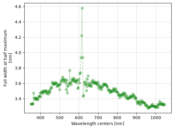
Calibrated Radiance True Color Image (Unorthorectified)
We select red (640 nm), green (550 nm), and blue (460 nm) bands to make a true-color image.
Because radiance values vary widely between bands, we apply a 2-98% percentile stretch to each band.
def stretch(band, lower=2, upper=98):
    """percentile stretch to the 0-1 range"""
    p_low, p_high = np.nanpercentile(band, [lower, upper])
    return np.clip((band - p_low) / (p_high - p_low), 0, 1)

rgb_wl = [640, 550, 460]
rgb_raw = rad['radiance'].sel(wavelength=rgb_wl, method='nearest').load()

rgb_raw_img = np.dstack([stretch(b) for b in rgb_raw.values])

fig, ax = plt.subplots(figsize=(7, 7))
ax.imshow(rgb_raw_img)
ax.set_xlabel('samples (across-track)')
ax.set_ylabel('lines (along-track)')
ax.set_title('PRISM Calibrated Radiance (True Color)')
plt.show()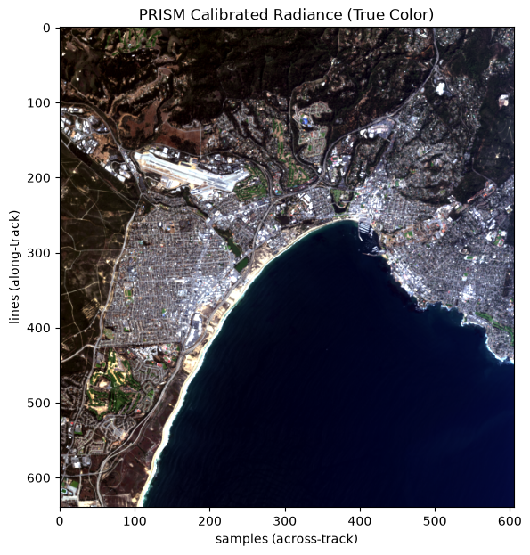
Note that the image above is not orthorectified.
Orthorectify with the Geometric Lookup Table
The GLT (geolocation_lookup_table) provides a grid in UTM coordinates. Each GLT pixel stores the raw line and sample of the pixel that falls there:
The function below uses the GLT to resample any raw array onto the UTM grid. It returns an xarray.DataArray with x/y coordinates and the CRS attached.
def orthorectify(data, glt, crs):
    # map a (..., lines, samples) raw-geometry array onto the GLT's UTM grid
    line = glt['line'].values
    sample = glt['sample'].values
    valid = ~np.isnan(line)
    # lines/samples starts with 1
    # subtracting 1 to convert to 0-based index
    # converting both -ve/+ve values to absolute
    li = np.abs(line[valid]).astype(int) - 1
    si = np.abs(sample[valid]).astype(int) - 1

    data = np.asarray(data)
    out = np.full(data.shape[:-2] + line.shape,
                  np.nan, dtype=np.float32)
    out[..., valid] = data[..., li, si]

    da = xr.DataArray(out, dims=('band', 'y', 'x'),
                      coords={'y': glt['northing'].values,
                              'x': glt['easting'].values})
    return da.rio.write_crs(crs)

rgb_ortho = orthorectify(rgb_raw.values, glt, crs)
rgb_ortho = rgb_ortho.assign_coords(band=rgb_raw['wavelength'].values)
rgb_orthoNow we plot the raw and orthorectified images side by side.
rgb_ortho_img = np.dstack([stretch(b) for b in rgb_ortho.values])
# show pixels outside the swath as white
rgb_ortho_img[np.isnan(rgb_ortho.values[0])] = 1

fig, axes = plt.subplots(1, 2, figsize=(15, 7))
axes[0].imshow(rgb_raw_img)
axes[0].set_title('PRISM Radiance (Unorthorectified) True Color RGB')
axes[0].set_xlabel('Samples')
axes[0].set_ylabel('Lines')

extent = [float(rgb_ortho.x.min()), float(rgb_ortho.x.max()),
          float(rgb_ortho.y.min()), float(rgb_ortho.y.max())]
axes[1].imshow(rgb_ortho_img, extent=extent)
axes[1].set_title(f"PRISM Radiance (Orthorectified {crs.name}) True Color RGB")
axes[1].set_xlabel('Easting (m)')
axes[1].set_ylabel('Northing (m)')
plt.tight_layout()
plt.show()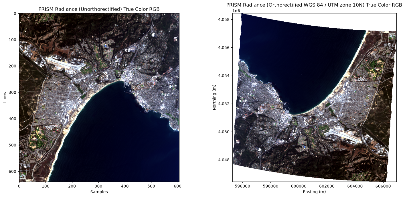
Map the Orthorectified Image
Because the orthorectified image has a CRS, we can plot it on a basemap. We will use cartopy in the PRISM data’s native UTM projection to avoid resampling.
# add an alpha band for transparent pixels for nan
swath = ~np.isnan(rgb_ortho.values[0])
rgba = np.dstack([rgb_ortho_img, swath.astype(float)])

# UTM projection
proj = ccrs.epsg(crs.to_epsg())
tiles = cimgt.GoogleTiles(url=xyz)

# buffer of 1.5 km around image
pad = 1500
map_extent = [extent[0] - pad, extent[1] + pad,
              extent[2] - pad, extent[3] + pad]

# plot
fig = plt.figure(figsize=(10, 10))
ax = plt.axes(projection=proj)
ax.set_extent(map_extent, crs=proj)
ax.add_image(tiles, 12)
ax.imshow(rgba, extent=extent, origin='upper', transform=proj, zorder=2)
gl = ax.gridlines(draw_labels=True, alpha=0.3)
gl.top_labels = gl.right_labels = False
ax.set_title(f'PRISM Corrected Radiance True Color RGB\n{granule_name}')
plt.show()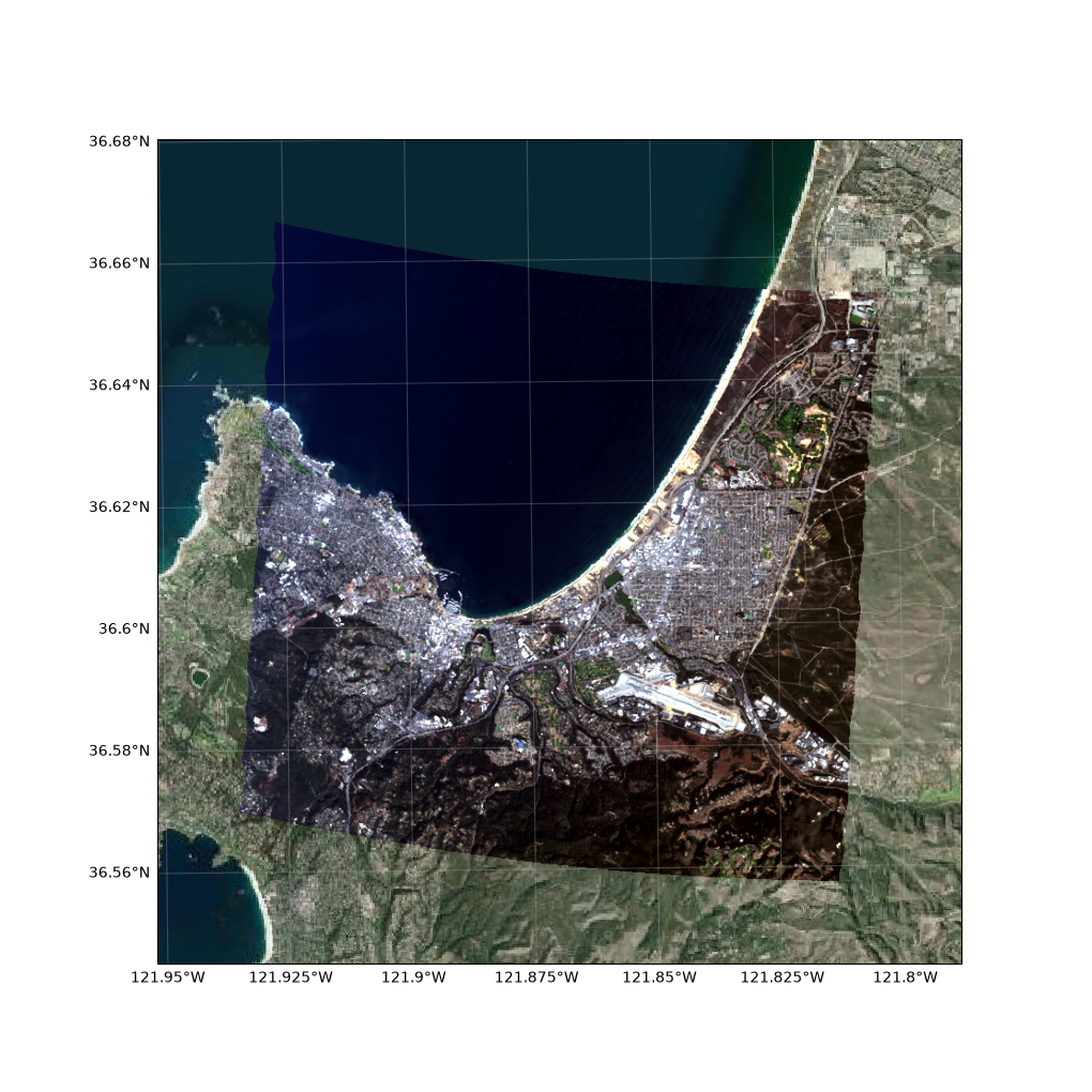
Radiance Spectra
Let’s extract radiance spectra for four surface types - one each for open water, beach, vegetation, and urban surface.
# points of interest (latitude, longitude)
points = {
    'Open water': (36.625, -121.87),
    'Beach sand': (36.623, -121.847),
    'Vegetation': (36.565, -121.850),
    'Urban': (36.612, -121.848),
}

lat = root['lat'].values
lon = root['lon'].values

spectra = {}
for name, (plat, plon) in points.items():
    # nearest pixel
    dist = (lat - plat)**2 + ((lon - plon) * np.cos(np.radians(plat)))**2
    i, j = np.unravel_index(np.nanargmin(dist), dist.shape)
    spectra[name] = rad['radiance'].isel(lines=i, samples=j).values
    print(f"{name:<12} line={i:<4} sample={j:<4}")
Open water line=424 sample=309
Beach sand line=424 sample=193
Vegetation line=36 sample=183
Urban line=352 sample=194
We plot the radiance spectra using pandas plot feature.
units = rad['radiance'].attrs['units']
spec_df = pd.DataFrame(spectra)
spec_df['Wavelength']=wl
spec_df.set_index('Wavelength', inplace=True)
spec_df.plot(marker="o", alpha=0.3, figsize=(10, 5),
            title='PRISM L1B Calibrated Radiance Spectra',
            ylabel=f"Radiance ({units})")
plt.grid(linestyle="--", alpha=0.5)
plt.show()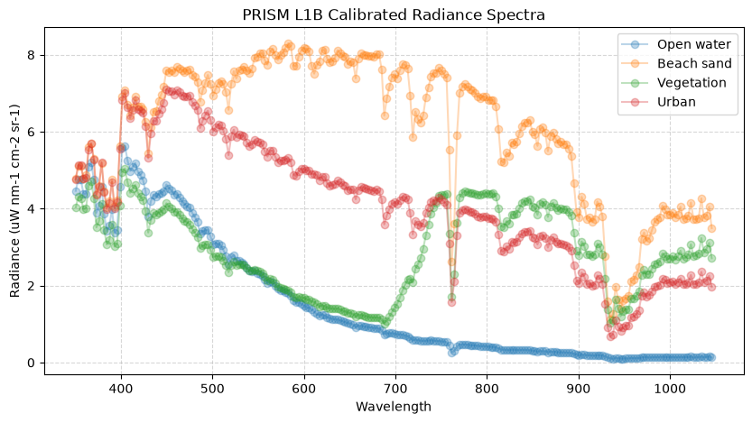
In the above calibrated radiance spectral plot, open water is brightest in the blue and decreases toward the near infrared (NIR), where water absorbs almost all light. Vegetation shows the red edge, a sharp rise in radiance between ~680 and ~750 nm caused by chlorophyll absorption in the red and strong leaf scattering in the NIR. Sand and urban surfaces are bright across the spectrum.
Export an Orthorectified GeoTIFF
The orthorectified array has a CRS and coordinates, so rioxarray can write it directly to a Cloud Optimized GeoTIFF (COG) for use in GIS software. As an example, here we export the orthorectified RGB true-color radiance bands.
out_tif = f"{granule_name}_RGB_ortho.tif"
rgb_ortho.rio.write_nodata(np.nan).rio.to_raster(out_tif, driver='COG')
print(f"Saved: {out_tif}")
Saved: PACEPAX-PRISM-L1B_ER2_20240926181605_R0_019.nc_RGB_ortho.tif
PACE OCI Surface Reflectance
PACE-PAX was designed to validate the Ocean Color Instrument (OCI) on the NASA PACE satellite. PRISM PACE-PAX reflectance dataset is not yet published. Therefore, we use the OCI reflectance of the same four locations, from the PACE OCI Level-2 Regional Surface Reflectance, Version 3.1 dataset (PACE_OCI_L2_SFREFL). The dataset provides the surface reflectance (rhos), corrected for the atmosphere, over both land and water, for 122 bands between 346 and 2258 nm. OCI pixels are about 1.2 km across at nadir, compared to ~18 m for PRISM in this scene.
Note that the PRISM data above are calibrated radiance at the sensor, while the OCI data are surface reflectance, so the values cannot be compared directly. The spectral shapes of the surfaces can be compared.
Search for the OCI granule
We search for OCI granules acquired on the same day as the PRISM scene, over the bounding box of the four points.
# PRISM acquisition time
prism_time = pd.to_datetime(dt.attrs['time_coverage_start'])
prism_date = prism_time.strftime('%Y-%m-%d')

# bounding box (west, south, east, north) of the four points
pt_lats = [p[0] for p in points.values()]
pt_lons = [p[1] for p in points.values()]
pts_bbox = (min(pt_lons), min(pt_lats), max(pt_lons), max(pt_lats))

pace_granules = earthaccess.search_data(short_name='PACE_OCI_L2_SFREFL', version='3.1',
                                        bounding_box=pts_bbox,
                                        temporal=(prism_date, prism_date))
for g in pace_granules:
    pace_time = pd.to_datetime(g['umm']['TemporalExtent']['RangeDateTime']['BeginningDateTime'])
    print(f"{g['umm']['GranuleUR']} => {(pace_time - prism_time).total_seconds() / 3600:+.1f} hours from PRISM")
PACE_OCI_L2_SFREFL_PACE_OCI.20240926T202511.L2.SFREFL.V3_1.nc_3.1 => +1.9 hours from PRISM
The OCI overpass was about two hours after the PRISM flight line. Each OCI L2 granule covers about 5 minutes of the orbit. Let’s open the pace granules with earthaccess.
pace_f = earthaccess.open(pace_granules[:1])[0]
pace_dt = xr.open_datatree(pace_f, engine='h5netcdf')
pace_dtThe OCI L2 file has these relevant groups and variables, which we can combine into one convenient xarray dataset using xr.merge():
| Group | Variables | Description |
|---|---|---|
/geophysical_data | rhos, l2_flags | Surface reflectance with dimensions (number_of_lines, pixels_per_line, wavelength_3d), and quality flags for each pixel |
/navigation_data | latitude, longitude | Location of each pixel center in the swath |
/sensor_band_parameters | wavelength_3d | Center wavelength of each rhos band (nm) |
pace_ds = xr.merge(
    (
        pace_dt.ds,
        pace_dt["geophysical_data"].to_dataset(),
        pace_dt["sensor_band_parameters"].coords,
        pace_dt["navigation_data"].ds.set_coords(("longitude", "latitude")).coords,
    )
)

# make 2D lat/lons selectable
pace_ds = pace_ds.set_xindex(("latitude", "longitude"), xr.indexes.NDPointIndex)

# add row, column numbers for each pixel to track pixel index
pace_ds = pace_ds.assign_coords(
    line_idx=("number_of_lines", np.arange(pace_ds.sizes["number_of_lines"])),
    pixel_idx=("pixels_per_line", np.arange(pace_ds.sizes["pixels_per_line"]))
)

pace_dsNote that like the PRISM L1B data, the OCI L2 data are in the swath geometry of the sensor.
print(f"Swath size (lines, pixels): {pace_ds["latitude"].shape}, bands: {pace_ds["wavelength_3d"].size}" \
      f" ({pace_ds["wavelength_3d"].min():.0f}-{pace_ds["wavelength_3d"].max():.0f} nm)")
Swath size (lines, pixels): (1710, 1272), bands: 122 (346-2258 nm)
Extract OCI reflectance at the four points
For each point, we find the nearest OCI pixel, as we did for PRISM, and read its reflectance spectrum. We also decode the l2_flags of the pixel. Each bit of l2_flags is a flag, and the flag names are stored in the flag_meanings attribute.
flag_names = pace_ds["l2_flags"].attrs['flag_meanings'].split()
flag_bits = pace_ds["l2_flags"].attrs['flag_masks']

def decode_flags(value):
    """returns the names of the flags set in an l2_flag."""
    return [n for n, b in zip(flag_names, flag_bits) if int(value) & int(b)]

pace_spectra = {}
rows = []
for name, (plat, plon) in points.items():
    # select a point from the full PACE dataset
    pace_point = pace_ds.sel(latitude=plat, longitude=plon, method="nearest")

    # distance (km) from the point to each OCI pixel center
    dist = np.hypot((pace_point["latitude"] - plat) * 111.32,
                    (pace_point["longitude"] - plon) * 111.32 * np.cos(np.radians(plat)))

    pace_spectra[name] = pace_point["rhos"].values

    rows.append({'location': name,
                 'line': pace_point.line_idx.item(),
                 'pixel': pace_point.pixel_idx.item(),
                 'distance_km': round(float(dist.values), 2),
                 'flags': ', '.join(decode_flags(pace_point["l2_flags"].values))})
pd.DataFrame(rows)Each point falls in a different OCI pixel, within ~0.6 km of the pixel center. A few flags are set:
LAND: the pixel is over land.COASTZ: the pixel is in shallow coastal water.STRAYLIGHT: the pixel is close to bright pixels, such as land or clouds, and light scattered inside the instrument may affect it.CLDICE: the pixel was classified as cloud or ice. The beach pixel contains sand, surf, water, and town. Its brightness likely triggered the cloud test, but we cannot rule out a real cloud from these data alone.
Unlike PRISM, an OCI pixel does not contain only beach sand or only urban surface. At 1.2 km, every pixel near the coast is a mix of surfaces.
Map the OCI pixels
To see the difference in resolution, we map an OCI true-color image (red 645 nm, green 555 nm, blue 465 nm) around the four points. Each colored cell is one OCI pixel. The black rectangle is the extent of the PRISM scene.
# OCI swath window around the points
d0 = np.hypot((pace_ds["latitude"] - pt_lats[0]) * 111.32,
              (pace_ds["longitude"] - pt_lons[0]) * 111.32 * np.cos(np.radians(pace_ds["latitude"])))
i0, j0 = np.unravel_index(np.nanargmin(d0), d0.shape)
win = (slice(i0 - 15, i0 + 15),
       slice(j0 - 15, j0 + 15))
bands = [int(np.abs(pace_ds["wavelength_3d"].values - w).argmin()) for w in [645, 555, 465]]
pace_rgb = np.clip(pace_ds["rhos"][win[0], win[1], bands].values / 0.15, 0, 1)

fig, ax = plt.subplots(figsize=(8, 8))
ax.pcolormesh(pace_ds["longitude"][win], pace_ds["latitude"][win],
              np.nan_to_num(pace_rgb, nan=1), shading='nearest')
for (name, (plat, plon)), c in zip(points.items(), plt.cm.tab10.colors):
    ax.plot(plon, plat, 'o', color=c, mec='white', ms=10, label=name)
# PRISM scene extent
lat_p, lon_p = root['lat'].values, root['lon'].values
ax.add_patch(plt.Rectangle((np.nanmin(lon_p), np.nanmin(lat_p)),
                           np.nanmax(lon_p) - np.nanmin(lon_p),
                           np.nanmax(lat_p) - np.nanmin(lat_p),
                           fill=False, ec='k', lw=1.5, label='PRISM scene extent'))
ax.set_xlim(np.nanmin(lon_p) - 0.05, np.nanmax(lon_p) + 0.05)
ax.set_ylim(np.nanmin(lat_p) - 0.05, np.nanmax(lat_p) + 0.05)
ax.set_aspect(1 / np.cos(np.radians(np.mean(pt_lats))))
ax.set_xlabel('Longitude')
ax.set_ylabel('Latitude')
ax.set_title(f"PACE OCI L2 surface reflectance, true color\n{pace_granules[0]['umm']['GranuleUR'][19:]}")
ax.legend(loc='lower left')
plt.show()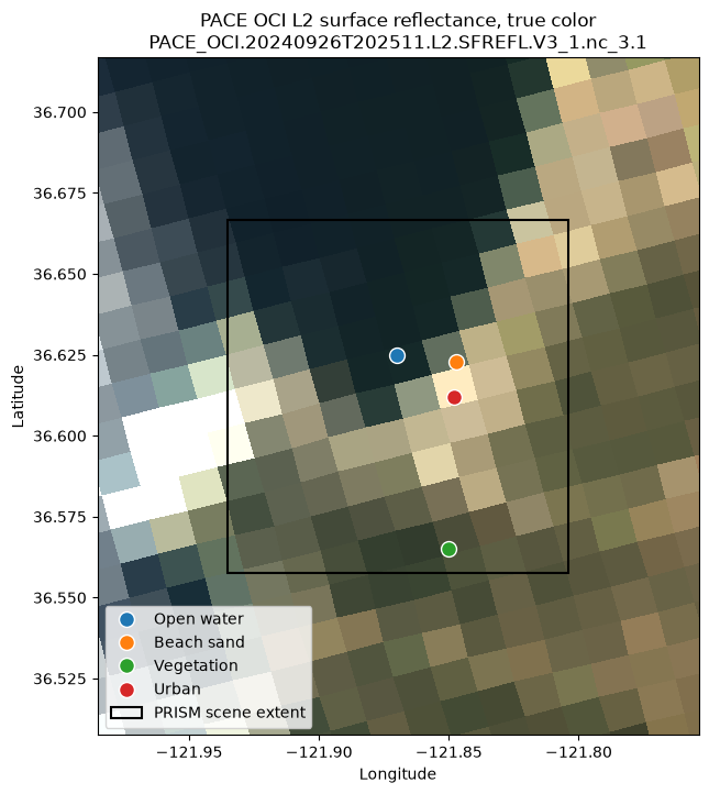
Plot the reflectance spectra
We plot the OCI reflectance spectra of the four points next to the PRISM radiance spectra from above. OCI also has seven shortwave infrared (SWIR) bands between 940 and 2258 nm, which PRISM does not cover. To compare the two, we plot only the OCI bands within the PRISM wavelength range, and use the same x-axis for both plots.
pace_df = pd.DataFrame(pace_spectra, index=pd.Index(pace_ds["wavelength_3d"].values, name='Wavelength'))
# keep only the OCI bands within the PRISM wavelength range
pace_df = pace_df[(pace_df.index >= float(wl.min())) & (pace_df.index <= float(wl.max()))]

fig, axes = plt.subplots(1, 2, figsize=(16, 5))
spec_df.plot(ax=axes[0], marker='o', ms=3, alpha=0.5,
             title='PRISM L1B radiance (~18 m pixels)', ylabel=f"Radiance ({units})")
pace_df.plot(ax=axes[1], marker='o', ms=3, alpha=0.5,
             title='PACE OCI L2 surface reflectance (~1.2 km pixels)', ylabel='Surface reflectance')
for ax in axes:
    ax.set_xlim(float(wl.min()), float(wl.max()))
    ax.grid(linestyle='--', alpha=0.5)
plt.tight_layout()
plt.show()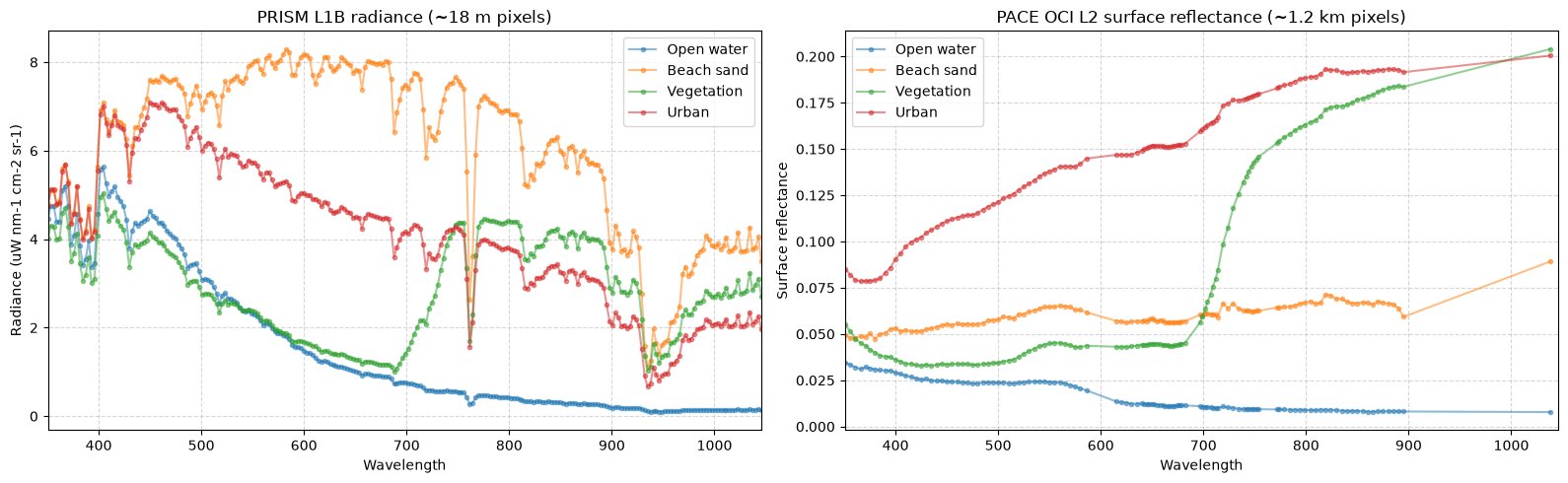
The OCI spectra show the same broad features as the PRISM spectra:
Open water is brightest in the blue and drops to almost zero in the NIR.
Vegetation shows the red edge between ~680 and ~750 nm.
The beach sand and urban spectra differ more from PRISM likely because of the difference in pixel size. The beach is a strip of sand a few tens of meters wide. At ~18 m, PRISM resolves it, and the sand is the brightest of the four surfaces. The OCI pixel at the beach is ~1.2 km across and mostly water, so its reflectance is low (0.05–0.07). It is also flagged CLDICE (cloud or ice). The OCI urban pixel, in contrast, includes bright town surfaces and is the brightest of the four.
- Mouroulis, P., Van Gorp, B., Green, R. O., Dierssen, H., Wilson, D. W., Eastwood, M., Boardman, J., Gao, B.-C., Cohen, D., Franklin, B., Loya, F., Lundeen, S., Mazer, A., McCubbin, I., Randall, D., Richardson, B., Rodriguez, J. I., Sarture, C., Urquiza, E., … Yee, K. (2014). Portable Remote Imaging Spectrometer coastal ocean sensor: design, characteristics, and first flight results. Applied Optics, 53(7), 1363. 10.1364/ao.53.001363
- Knobelspiesse, K. D., Cetinić, I., Cairns, B., Leblanc, S. E., & Ueyama, R. (2026). The NASA Plankton, Aerosol, Cloud, ocean Ecosystem mission Postlaunch Airborne eXperiment (PACE-PAX). 10.5194/essd-2026-541
- Bender, H., Brunner, E. D., Chapman, J. W., Coleman, R. W., Eastwood, M., Eckert, R., Gierach, M. M., Luis, K. M. A., Rios, L. M., Small, Z., & Thompson, D. R. (2026). PRISM: L1B Calibrated Radiance for PACE-PAX, 2024. ORNL Distributed Active Archive Center. 10.3334/ORNLDAAC/2515
- NASA Ocean Biology Processing Group. (2025). PACE OCI Level-2 Regional Surface Reflectance Data, version 3.1. NASA Ocean Biology Distributed Active Archive Center. 10.5067/PACE/OCI/L2/SFREFL/3.1