Overview
The MODIS/ASTER Airborne Simulator (MASTER) Level 2 (L2) dataset provides land surface temperature (LST) and emissivity derived from the instrument’s thermal infrared (TIR) bands. Unlike the L1B radiance data, which is organized as one data collection per campaign, the L2 product is a cross-campaign Facility Instrument Collection that aggregates standardized L2 retrievals from all MASTER deployments since 1998.
L2 retrievals use the ASTER Temperature-Emissivity Separation (TES) algorithm combined with the MODTRAN radiative transfer model for atmospheric correction. Emissivity is retrieved in six TIR bands spanning 8.58–12.13 µm. L2 files are distributed in HDF-5 format.
In this tutorial we use earthaccess to discover and access MASTER L2 data and then visualize land surface temperature and emissivity.
Datasets Used
| Dataset | DOI | Concept ID |
|---|---|---|
| MASTER: Level 2 Emissivity and Land Surface Temperature | Hulley et al. (2026) | C4092063695-ORNL_CLOUD |
Learning Objectives
Search the MASTER L2 Facility Instrument Collection using campaign keyword
Stream a HDF-5 L2 granule directly from the Earthdata Cloud using
earthaccessandxarrayExplore the HDF-5 file structure and read and visualize LST and emissivity variables
Prerequisites
A free NASA Earthdata Login account is required. See the prerequisites page for setup instructions.
Import Libraries
import earthaccess
import xarray
import numpy as np
import matplotlib.pyplot as plt
import geopandas as gpd
import pandas as pd
import cartopy.crs as ccrs
import cartopy.io.img_tiles as cimgt
import warnings
warnings.filterwarnings('ignore')

xyz = "https://server.arcgisonline.com/ArcGIS/rest/services/World_Imagery/MapServer/tile/{z}/{y}/{x}"
attr = "ESRI"Authentication
Use earthaccess.login() to authenticate with your NASA Earthdata Login credentials. If you have a .netrc file configured, login will complete without prompting.
auth = earthaccess.login()Search the MASTER L2 Collection
The MASTER Level 2 Facility Instrument Collection (doi:10.3334/ORNLDAAC/2489) aggregates L2 retrievals from all MASTER campaigns. We can search the granules directly using earthaccess.
# Search for the MASTER L2 Facility Instrument Collection
collections = earthaccess.search_datasets(
    doi='10.3334/ORNLDAAC/2489'
)

print(f"Collections found: {len(collections)}")
for c in collections:
    # file dist. info
    fdi = c.get_umm('ArchiveAndDistributionInformation')['FileDistributionInformation'][0]
    print(f"  Title    : {c.get_umm('EntryTitle')}")
    print(f"  ShortName: {c.get_umm('ShortName')}")
    print(f"  ConceptID: {c.concept_id()}")
    print(f"  Version  : {c.get_umm('Version')}")
    print(f"  File Size  : {fdi['TotalCollectionFileSize']} {fdi['TotalCollectionFileSizeUnit'] }")
    print(f"  File format  : {fdi['Format']}")
    print(f"  Citation : {c.citation(format='apa',language="en-US")}")
Collections found: 1
Title : MASTER: Level 2 Emissivity and Land Surface Temperature
ShortName: MASTER_L2_Emiss_LST_2489
ConceptID: C4092063695-ORNL_CLOUD
Version : 1
File Size : 538.973 GB
File format : HDF5
Citation : Hulley, G. C., Hook, S. J., La, T. T., & Rivera, G. (2026). MASTER: Level 2 Emissivity and Land Surface Temperature (Version 1). ORNL Distributed Active Archive Center. https://doi.org/10.3334/ORNLDAAC/2489
Search for L2 granules for a project
We search for L2 granules within for NASA’s GEMx project. The Geological Earth Mapping Experiment (GEMx) is a joint campaign between NASA and the U.S. Geological Survey (USGS) to map portions of the western United States for critical minerals using advanced airborne imaging, inclding AVIRIS and MASTER instruments.
# dataset short name
short_name='MASTER_L2_Emiss_LST_2489'
# project name
project = 'GEMx'

# earthaccess query
query = earthaccess.DataGranules().short_name(short_name)
query.params['campaign'] = project
granules = query.get_all()

print(f"Granules found for {project} project: {len(granules)}")
Granules found for GEMx project: 665
Let’s inspect the first granule.
granules[0]Explore L2 Granule Footprints
We convert granule metadata into a geopandas dataframe.
gdf = gpd.GeoDataFrame(pd.json_normalize(granules),
                                geometry=gpd.GeoSeries(granules, crs=4326))
gdfLet’s first plot time range of the granules collected for the NASA GEMx campaign.
gdf['dt'] = pd.to_datetime(gdf['umm.TemporalExtent.RangeDateTime.BeginningDateTime'])
# montly bins
gdf['month_year'] = gdf['dt'].dt.strftime('%Y-%m')
# Group and count occurrences per interval
gdf.groupby('month_year').size().plot(kind='bar',
                                     edgecolor='black')
plt.xlabel('Flight Dates')
plt.ylabel('Number of granules')
plt.title((
    f"""MASTER Level 2 Granules for {project} project
    between {gdf['dt'].min().date()} and {gdf['dt'].max().date()}"""
    ))
plt.tight_layout()
plt.show()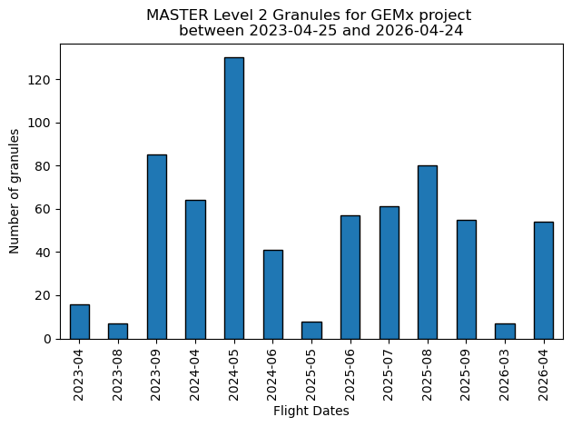
As we can see in the above chart, several MASTER flights were flown for GEMx campaign during 2003-2026.
Now, we can also plot the granule boundaries in a map.
gdf['year'] = gdf['dt'].dt.strftime('%Y')
gdf[['meta.native-id', 'year', 'geometry']].explore(
    tiles=xyz, attr=attr, column="year",
    style_kwds={"weight": 2, "fillOpacity": 0.1},
)Export granule bounds for GIS
The granule information can also be exported to a GeoJSON format and imported into a GIS software.
gdf.to_file("granule.geojson", driver="GeoJSON")Open a L2 Granule from the Cloud
MASTER L2 files are in HDF-5 format. We use earthaccess.open() to obtain the file-like objects and read them directly with xarray, not needing local download.
# Open the first granule as a cloud-streamed file object
file_objs = earthaccess.open([granules[0]])
granule0 = granules[0].get('umm',[]).get('GranuleUR',[])
print(f"Opened granule: {granule0}")Opened granule: MASTERL2_2364900_01_20230425_1733_1751_V02_B200_SV01.hdf5
# xarray can read from a file-like object directly
ds = xarray.open_dataset(file_objs[0], chunks={})
dsExplore the file structure
Let’s list all the variables and dimensions of the datasest. The dataset has four variables Emissivity, LST, Lat, Lon and QAmap.
ds.info()xarray.Dataset {
dimensions:
phony_dim_0 = 6738 ;
phony_dim_1 = 716 ;
phony_dim_2 = 6 ;
variables:
float32 Emissivity(phony_dim_0, phony_dim_1, phony_dim_2) ;
Emissivity:description = Atmospheric Corrected MASTER Emissivity - TES corrected bands ;
Emissivity:wavelength = [ 8.3 8.61 9.04 10.62 11.32 12.13] ;
Emissivity:wavelength units = Micrometers ;
float32 LST(phony_dim_0, phony_dim_1) ;
LST:band names = LST (K) ;
LST:description = Temperature (K) - TES LST ;
float32 Lat(phony_dim_0, phony_dim_1) ;
Lat:description = Latitude ;
Lat:units = degrees ;
float32 Lon(phony_dim_0, phony_dim_1) ;
Lon:description = Longitude ;
Lon:units = degrees ;
float32 QAmap(phony_dim_0, phony_dim_1) ;
QAmap:description = QA data from TES algorithm: 1 is divergence, 0 is convergence ;
// global attributes:
:Build = 200 ;
:HDF5_Version = 1.14.2 ;
:Software Version = 01 ;
:acquisition_time = 2023-04-25 17:33:04 ;
:description = Atmospheric Corrected MASTER Land Surface Temperature (Kelvin), Emissivity - TES corrected bands (Micrometers), and QAmap (1 - divergence, 0 - convergence) ;
:h5py_version = 3.10.0 ;
:modification_time = 2025-06-03 02:42:53 ;
}Assign Coordinates
Lat and Lon variables provide per-pixel geolocation. Let’s assigned them as the coordinates for the dataset so we can use it later for plotting.
ds = ds.assign_coords(lon=ds.Lon, lat=ds.Lat)
dsLand Surface Temperature
The LST variable holds per-pixel surface temperature in Kelvin.
ds.LSTNow, Let’s print minimum and maximum LST values.
print(f"LST range (K): {float(ds.LST.min()):.2f} – {float(ds.LST.max()):.2f}")LST range (K): 292.20 – 433.70
We display the LST variable in degrees Celsius in the following, where surface temperature is represented from cool (dark) to hot (bright).
# OpenStreet baselayers
request = cimgt.OSM()

fig = plt.figure(figsize=(10, 8))
ax = plt.axes(projection=request.crs)

# baselayer zoom
ax.add_image(request, 9)

# K to C
lst_celsius = ds.LST - 273.15
# setting min max
vmin, vmax = np.nanpercentile(lst_celsius, [2, 98])
im = lst_celsius.plot(
        ax=ax, x='lon', y='lat',
        vmin=vmin, vmax=vmax,
        transform=ccrs.PlateCarree(),
        cmap='inferno', add_colorbar=False
)
ax.set_title(f"MASTER L2 Land Surface Temperature {granule0}", fontsize=13)
fig.colorbar(im, ax=ax, label=f"LST (Celsius)", pad=0.05, shrink=0.7)
plt.show()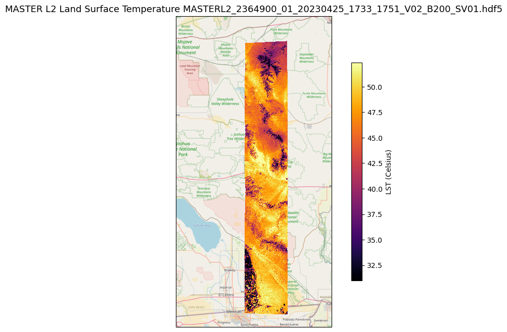
Emissivity
The TES algorithm retrieves emissivity in six thermal infrared (TIR) bands corresponding to spectral regions between 8.3 and 12.11 µm. Emissivity values are dimensionless (0–1), where 1.0 is a perfect blackbody.
ds.EmissivityLet’s print minumum and maximum emissivity values for each of the 6 bands
# MASTER TIR emissivity band center wavelengths (µm) for the 6 retrieved bands
wavelengths = ds.Emissivity.attrs.get("wavelength",[])

for i, wl in enumerate(wavelengths):
    emiss = ds.Emissivity.isel({'phony_dim_2': i})
    print(f"Emissivity range for Band {wl} µm:  {float(emiss.min()):.2f} – {float(emiss.max()):.2f}")
Emissivity range for Band 8.3 µm: 0.68 – 1.00
Emissivity range for Band 8.61 µm: 0.69 – 0.99
Emissivity range for Band 9.04 µm: 0.64 – 0.99
Emissivity range for Band 10.62 µm: 0.77 – 0.99
Emissivity range for Band 11.32 µm: 0.67 – 0.99
Emissivity range for Band 12.13 µm: 0.60 – 0.99
Now, let’s visualize all six retrieved emissivity bands. Emissivity near 1.0 indicates a near-perfect blackbody. Water and dense vegetation have higher emissivity values. Lower emissivity values are typical of bare soils, rocks, and deserts.
# OpenStreet baselayers
request = cimgt.OSM()

fig, axes = plt.subplots(
    nrows=2, ncols=3, figsize=(16, 10),
    subplot_kw={'projection': request.crs})
axes = axes.flatten()

for i, wl in enumerate(wavelengths):
    emiss = ds.Emissivity.isel({'phony_dim_2': i})
    vmin, vmax = np.nanpercentile(emiss, [2, 98])
    axes[i].add_image(request, 9)

     # plot one band
    im = emiss.plot(
        ax=axes[i], x='lon', y='lat', transform=ccrs.PlateCarree(),
        cmap='RdYlGn', vmin=vmin, vmax=vmax,add_colorbar=False
    )

    axes[i].set_title(f"Emissivity - {wl} µm", fontsize=10)
    fig.colorbar(im, ax=axes[i], label="Emissivity", pad=0.05, shrink=0.7)


plt.suptitle(f"MASTER L2 Emissivity {granule0}", fontsize=13)
plt.tight_layout()
plt.show()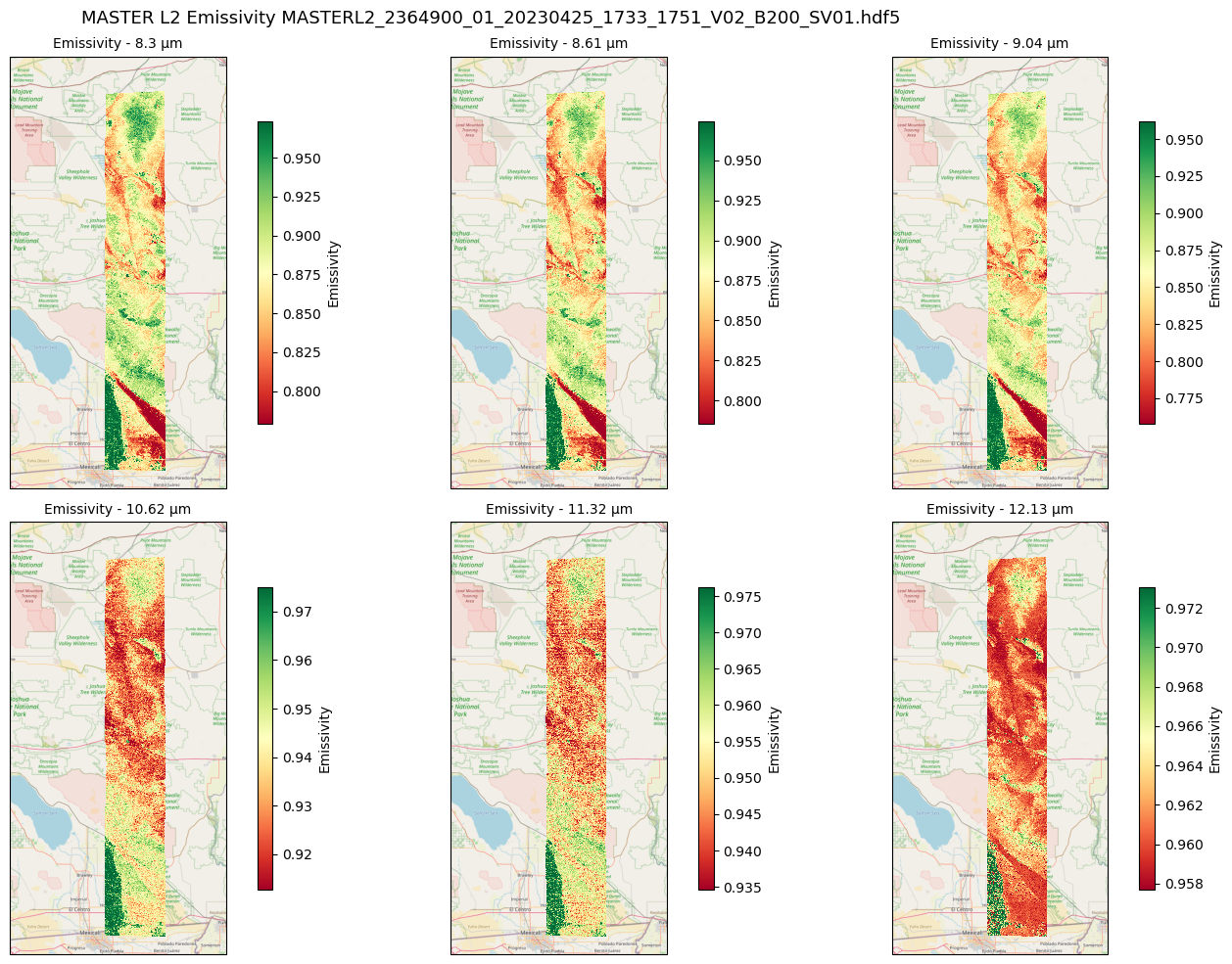
Emissivity for a Selected Pixel
We select the pixel with the highest LST (hot, dry surface) and a second pixel with the lowest LST for comparing how emissivity varies across the bands.
def get_idx(flat_idx, ds_shape, ds_dims):
    """converts flat index into multidimensional index."""
    grid_indices = np.unravel_index(flat_idx, ds_shape)
    return {dim: idx for dim, idx in zip(ds_dims, grid_indices)}

# lst layer
lst = ds.LST.compute()

# flattened index of min value
min_idx = get_idx(lst.argmin(dim=None).item(),
                  lst.shape, lst.dims)
max_idx = get_idx(lst.argmax(dim=None).item(),
                  lst.shape, lst.dims)

plt.figure(figsize=(10, 5))

# emissivity at min max LST plots
ds.Emissivity.isel(min_idx).plot(
    label=f"Cold Pixel, LST {lst[min_idx]:.1f} K",
    ls="--", marker="o", color="steelblue"
)
ds.Emissivity.isel(max_idx).plot(
    label=f"Hot Pixel, LST {lst[max_idx]:.1f} K",
    marker="s", color="firebrick"
)
plt.xticks(ticks=np.arange(len(wavelengths)), labels=wavelengths)
plt.xlabel("Wavelength µm")
plt.title(f"MASTER L2 Emissivity {granule0}")
plt.grid(True, linestyle=":", alpha=0.6)
plt.legend()
plt.show()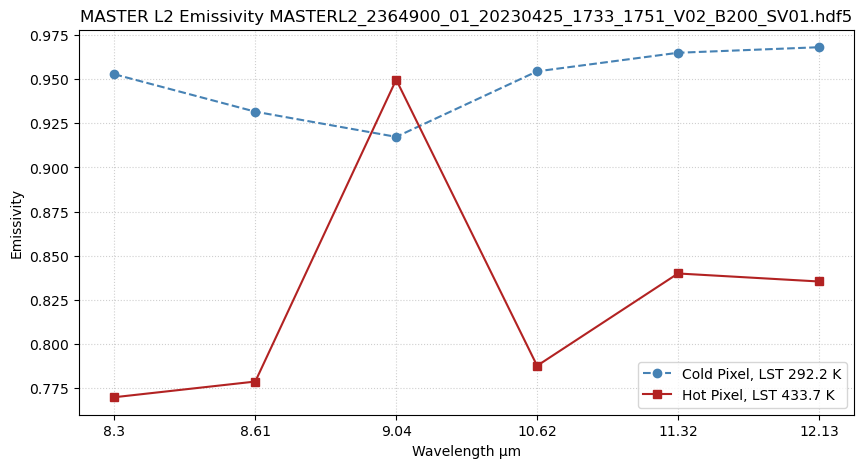
For access to the underlying L1B calibrated radiance used to derive these L2 products, see the MASTER L1B notebook.
- Hulley, G. C., Hook, S. J., La, T. T., & Rivera, G. (2026). MASTER: Level 2 Emissivity and Land Surface Temperature. ORNL Distributed Active Archive Center. 10.3334/ORNLDAAC/2489