Access and Visualization of MASTER L1B Radiance Data - NASA Airborne Science Data Tutorials

Overview¶

The MODIS/ASTER Airborne Simulator (MASTER) is a multispectral scanning spectrometer that collects calibrated radiance across 50 spectral channels spanning 0.46 to 12.879 micrometers — covering the visible, near-infrared, shortwave infrared, and thermal infrared portions of the electromagnetic spectrum. MASTER has flown since 1998 on a variety of NASA aircraft as a Facility Instrument of the NASA Airborne Science Program.

In this tutorial we use earthaccess to discover and access MASTER Level 1B (L1B) calibrated radiance data from the Western Diversity Time Series (WDTS) Spring 2024 campaign. The WDTS campaign observes California’s ecosystems and supports monitoring of natural hazards such as wildfires, volcanoes, and drought.

MASTER L1B files are georeferenced multispectral images in HDF-4 format, archived as individual flight-line granules at the ORNL DAAC.

Datasets Used¶

Dataset	DOI	Concept ID
MASTER: Western Diversity Time Series Campaign, WDTS, Spring 2024	Hook et al. (2024)	C3323041261-ORNL_CLOUD

Learning Objectives¶

Search NASA CMR for a MASTER campaign collection by short name
List and filter granules by spatial bounding box and date range using earthaccess
Download a HDF-4 L1B granule and explore its file structure and extract a radiance band
Visualize a selected MASTER radiance band

Prerequisites¶

A free NASA Earthdata Login account is required. See the prerequisites page for setup instructions.

Import Libraries¶

import earthaccess
import numpy as np
import matplotlib.pyplot as plt
import geopandas as gpd
import pandas as pd
import pyhdf.SD as SD
import xarray
import cartopy.crs as ccrs
import cartopy.io.img_tiles as cimgt
import warnings
warnings.filterwarnings('ignore')

xyz = "https://server.arcgisonline.com/ArcGIS/rest/services/World_Imagery/MapServer/tile/{z}/{y}/{x}"
attr = "ESRI"

Authentication¶

Use earthaccess.login() to authenticate with your NASA Earthdata Login credentials. If you have a .netrc file configured, login will complete without a prompt.

auth = earthaccess.login()

Search for the MASTER WDTS Collection¶

Each MASTER campaign is archived as its own collection at the ORNL DAAC. We search by instrument and project to locate the Western Diversity Time Series (WDTS) L1B MASTER datasets.

# Search for the MASTER WDTS collections
collections = earthaccess.search_datasets(
    instrument="MASTER", # 
    project = "WDTS"
)

print(f"Collections found: {len(collections)}")
for c in collections:
    print(f"  Title    : {c.get_umm('EntryTitle')}")
    print(f"  ShortName: {c.get_umm('ShortName')}")

Collections found: 9
  Title    : MASTER: Flight Line Geospatial Polygons and Contextual Data
  ShortName: MASTER_Flightline_Locator_2151
  Title    : MASTER: Image Overlays for Level 2 Emissivity and Land Surface Temperature
  ShortName: MASTER_L2_Emiss_LST_Overlays_2487
  Title    : MASTER: Quicklook Images for Level 2 Emissivity and Land Surface Temperature
  ShortName: MASTER_L2_Emiss_LST_Quicklooks_2488
  Title    : MASTER: Western Diversity Time Series Campaign, WDTS, September 2022
  ShortName: MASTER_WDTS_Fall_2022_2141
  Title    : MASTER: Western Diversity Time Series Campaign, WDTS, California, USA, Fall 2020
  ShortName: MASTER_WDTS_SeptOct_2020_1940
  Title    : MASTER: Western Diversity Time Series Campaign, WDTS, California, USA, Spring 2021
  ShortName: MASTER_WDTS_Spring_2021_1953
  Title    : MASTER: Western Diversity Time Series Campaign, WDTS, Spring 2023
  ShortName: MASTER_WDTS_Spring_2023_2252
  Title    : MASTER: Western Diversity Time Series Campaign, WDTS, Spring 2024
  ShortName: MASTER_WDTS_Spring_2024_2383
  Title    : MASTER: Western Diversity Time Series Campaign, WDTS, Spring 2025
  ShortName: MASTER_WDTS_Spring_2025_2471

Search for Granules¶

We search for L1B flight-line granules from the WDTS 2024 campaign with ShortName as MASTER_WDTS_Spring_2024_2383. MASTER L1B granules are individual flight-line files covering a swath width of roughly 6–37 km depending on flight altitude.

Here, we search across the full campaign date range and filter by a bounding box over California.

# Bounding box: (west, south, east, north) — California/Nevada region
bbox = (-123.75, 31.95, -112.5, 40.98)

# Search granules from MASTER WDTS Spring 2024 L1B Collection
granules = earthaccess.search_data(
    short_name='MASTER_WDTS_Spring_2024_2383',
    bounding_box=bbox,
    temporal=('2024-06-04', '2024-06-28'),
)

print(f"Granules found: {len(granules)}")

Granules found: 336

Inspect Granule Metadata¶

We inspect the CMR granule metadata to identify file names and types before accessing any data.

# Build a DataFrame from granule metadata, first 25 granules
rows = [{'producer_granule_id': g['umm'].get('GranuleUR', '')} for g in granules[:25]]
df_granules = pd.DataFrame(rows)
print(df_granules[['producer_granule_id']].to_string(index=False))

                                                                  producer_granule_id
                           MASTER_WDTS_Spring_2024.MASTER_2495500_20240604_config.txt
          MASTER_WDTS_Spring_2024.MASTER_2495500_20240604_spectral_response_table.zip
              MASTER_WDTS_Spring_2024.MASTERL1B_2495500_01_20240604_1743_1757_V01.jpg
                        MASTER_WDTS_Spring_2024.MASTER_2495500_20240604_ancillary.txt
                          MASTER_WDTS_Spring_2024.MASTER_2495500_20240604_summary.txt
               MASTER_WDTS_Spring_2024.MASTER_2495500_20240604_spectral_band_info.txt
              MASTER_WDTS_Spring_2024.MASTERL1B_2495500_01_20240604_1743_1757_V01.hdf
                       MASTER_WDTS_Spring_2024.MASTER_2495500_20240604_flightpath.gif
         MASTER_WDTS_Spring_2024.MASTERL2_2495500_01_20240604_1743_1757_V01-QAmap.zip
MASTER_WDTS_Spring_2024.MASTERL2_2495500_01_20240604_1743_1757_V01-emissivity_tes.zip
      MASTER_WDTS_Spring_2024.MASTERL2_2495500_01_20240604_1743_1757_V01-location.zip
        MASTER_WDTS_Spring_2024.MASTERL2_2495500_01_20240604_1743_1757_V01-images.zip
  MASTER_WDTS_Spring_2024.MASTERL2_2495500_01_20240604_1743_1757_V01-surface_temp.zip
           MASTER_WDTS_Spring_2024.MASTERL2_2495500_01_20240604_1743_1757_V01-LST.kmz
              MASTER_WDTS_Spring_2024.MASTERL1B_2495500_02_20240604_1802_1816_V01.jpg
              MASTER_WDTS_Spring_2024.MASTERL1B_2495500_02_20240604_1802_1816_V01.hdf
         MASTER_WDTS_Spring_2024.MASTERL2_2495500_02_20240604_1802_1816_V01-QAmap.zip
           MASTER_WDTS_Spring_2024.MASTERL2_2495500_02_20240604_1802_1816_V01-LST.kmz
        MASTER_WDTS_Spring_2024.MASTERL2_2495500_02_20240604_1802_1816_V01-images.zip
      MASTER_WDTS_Spring_2024.MASTERL2_2495500_02_20240604_1802_1816_V01-location.zip
  MASTER_WDTS_Spring_2024.MASTERL2_2495500_02_20240604_1802_1816_V01-surface_temp.zip
MASTER_WDTS_Spring_2024.MASTERL2_2495500_02_20240604_1802_1816_V01-emissivity_tes.zip
              MASTER_WDTS_Spring_2024.MASTERL1B_2495500_03_20240604_1821_1835_V01.jpg
              MASTER_WDTS_Spring_2024.MASTERL1B_2495500_03_20240604_1821_1835_V01.hdf
  MASTER_WDTS_Spring_2024.MASTERL2_2495500_03_20240604_1821_1835_V01-surface_temp.zip

As we see above, MASTER L1B dataset has different file types. Please refer to the user guide for more information about the data files.

Map Flight Lines¶

We extract the footprint polygon from each granule’s spatial bounds and plot the flight lines over the region of interest.

# plot granule footprints over the study area
flight_paths_gdf = gpd.GeoDataFrame(granules, geometry=gpd.GeoSeries(granules, crs=4326))
flight_paths_gdf.geometry.explore(
    tiles=xyz, attr=attr, color="red",
    style_kwds={"weight": 2, "fillOpacity": 0.1},
    name="L1 Radiance Footprints",
)

Access an L1B Granule¶

MASTER L1B files are in HDF-4 format. We open the first granule directly from the Earthdata Cloud using earthaccess.open() which returns file-like objects that can be read without downloading to disk.

Because pyhdf requires a local file path, we download a granule using earthaccess.

# filter HDF granules only
g_hdfs = [g for g in granules if g.data_links()[0].endswith(".hdf")]

# Download the first granule from the cloud
downloaded = earthaccess.download(g_hdfs[0], local_path='data')
print(f"Granule download: {downloaded[0].as_posix()}")

Granule download: data/MASTERL1B_2495500_01_20240604_1743_1757_V01.hdf

Explore the HDF-4 File Structure¶

MASTER L1B HDF-4 files contain scientific datasets (SDSs) for each of the 50 spectral bands along with geolocation arrays. We list all available SDSs to understand the file layout. Please refer to the user guide for more information about the SDSs.

# Open the HDF-4 file
hdf = SD.SD(downloaded[0].as_posix(), SD.SDC.READ)

# list all Scientific Dataset (SDS) names and shapes
datasets = hdf.datasets()
print(f"{'SDS Name':<40}  {'Shape':>20}  {'Type':>8}")
print('-' * 75)
for name, (dims, shape_info, dtype, idx) in datasets.items():
    print(f"{name:<40}  {str(shape_info):>20}  {str(dtype):>8}")

SDS Name                                                 Shape      Type
---------------------------------------------------------------------------
Left50%ResponseWavelength                                (50,)         5
Central100%ResponseWavelength                            (50,)         5
Right50%ResponseWavelength                               (50,)         5
EffectiveCentralWavelength_IR_bands                      (50,)         5
TemperatureCorrectionSlope                               (50,)         5
TemperatureCorrectionIntercept                           (50,)         5
SolarSpectralIrradiance                                  (50,)         5
DataSetHeader                                        (149, 97)         4
ScanLineCounter                                        (5126,)        24
GreenwichMeanTime                                      (5126,)        24
YearMonthDay                                           (5126,)        24
AircraftRollCount                                      (5126,)        22
BlackBody1Temperature                                  (5126,)        22
BlackBody2Temperature                                  (5126,)        22
ScanRate                                               (5126,)         5
ScanlineTime                                           (5126,)         5
AircraftLatitude                                       (5126,)         6
AircraftLongitude                                      (5126,)         6
AircraftHeading                                        (5126,)         6
AircraftAltitude                                       (5126,)         6
AircraftPitch                                          (5126,)         6
TBack                                                  (5126,)         5
AnalogGain                                          (5126, 50)        22
AnalogOffset                                        (5126, 50)        22
BlackBody1Counts                                    (5126, 50)        23
BlackBody2Counts                                    (5126, 50)        23
Head1Counts                                         (5126, 50)        23
Head2Counts                                         (5126, 50)        23
CalibrationSlope                                    (5126, 50)         5
CalibrationIntercept                                (5126, 50)         5
PixelLatitude                                      (5126, 716)         6
PixelLongitude                                     (5126, 716)         6
PixelElevation                                     (5126, 716)         6
SensorZenithAngle                                  (5126, 716)         5
SensorAzimuthAngle                                 (5126, 716)         5
SolarZenithAngle                                   (5126, 716)         5
SolarAzimuthAngle                                  (5126, 716)         5
CalibratedData                                 (5126, 50, 716)        22

Read Radiance Bands¶

MASTER L1B data contains 50 calibrated radiance bands spanning visible through thermal infrared. Bands 1–25 cover the reflective solar spectrum; bands 26–50 cover the thermal infrared. We read several bands and inspect their statistics.

radiance_sds = 'CalibratedData'  # radiance SDS names
sds = hdf.select(radiance_sds)
radiance_shape = sds.dimensions()
print(f"Radiance SDS '{radiance_sds}' with dimensions: {sds.info()[2]}")

radiance = sds[:].astype(np.float32)
attrs = sds.attributes()
scale = attrs.get('scale_factor', 1.0)
fill  = attrs.get('_FillValue', -9999)
units = attrs.get('units', None)

# Apply scale factor and fill value 
radiance = np.where(radiance == fill, np.nan,
                    radiance * np.array(scale)[:, np.newaxis])

print(f"Radiance array shape: {radiance.shape}")
print(f"  scan lines × channels × pixels")
print(f"Min (non-nan): {np.nanmin(radiance):.4f} {units}")
print(f"Max (non-nan): {np.nanmax(radiance):.4f} {units}")

Radiance SDS 'CalibratedData' with dimensions: [5126, 50, 716]
Radiance array shape: (5126, 50, 716)
  scan lines × channels × pixels
Min (non-nan): -1.9200 watts/meter2/steradian/micron
Max (non-nan): 498.1000 watts/meter2/steradian/micron

Read Geolocation and Spectral Range¶

The latitude and longitude arrays in MASTER L1B files provide per-pixel geolocation for each scan line and sample. We read these to support georeferenced visualization.

# Read latitude and longitude arrays
lat_sds_name = 'PixelLatitude'
lon_sds_name = 'PixelLongitude'
# center wavelengths 
wv_sds_name = 'Central100%ResponseWavelength'

lat = hdf.select(lat_sds_name)[:].astype(np.float32)
lon = hdf.select(lon_sds_name)[:].astype(np.float32)
wv = hdf.select(wv_sds_name)[:].astype(np.float32)
    
# Mask fill values (typically -999 or 0 outside swath)
lat = np.where(lat < -90, np.nan, lat)
lon = np.where(lon < -180, np.nan, lon)
    
print(f"Lat range: {np.nanmin(lat):.4f} to {np.nanmax(lat):.4f}")
print(f"Lon range: {np.nanmin(lon):.4f} to {np.nanmax(lon):.4f}")
print(f"Spectral range: {np.nanmin(wv):.4f} to {np.nanmax(wv):.4f}")

Lat range: 36.6319 to 38.1581
Lon range: -119.1226 to -118.6993
Spectral range: 0.4620 to 12.8500

Band Statistics Summary¶

We compute per-band statistics across all 50 channels to understand the radiance range and identify any bands with fill data. Bands 1-25 are in visible–shortwave infrared (SWIR) region and bands 26–50 are in thermal infrared (TIR) region.

n_bands = wv.shape[0]
stats = []
for b in range(n_bands):
    band_data = radiance[:,b,:]
    valid = band_data[~np.isnan(band_data)]
    stats.append({
        'band': b + 1,
        'wavelength': wv[b],
        'min': np.nanmin(band_data) if len(valid) > 0 else np.nan,
        'max': np.nanmax(band_data) if len(valid) > 0 else np.nan,
        'mean': np.nanmean(band_data) if len(valid) > 0 else np.nan,
        'valid_pct': 100 * len(valid) / band_data.size
    })

df_stats = pd.DataFrame(stats)
print(df_stats.to_string(index=False, float_format='{:.3f}'.format))

 band  wavelength    min     max   mean  valid_pct
    1       0.462 32.300 498.100 89.641    100.000
    2       0.500 24.100 493.400 82.208    100.000
    3       0.544 18.200 495.400 81.628    100.000
    4       0.582 13.500 456.100 74.555    100.000
    5       0.654  8.300 388.100 64.248    100.000
    6       0.714  7.500 338.500 66.012    100.000
    7       0.752  5.400 280.300 69.473    100.000
    8       0.802  4.800 249.700 69.358    100.000
    9       0.868  3.500 194.000 59.810    100.000
   10       0.908  3.000 146.200 46.744    100.000
   11       0.948  2.500  93.500 28.968    100.000
   12       1.602  0.504  48.024 11.607    100.000
   13       1.660  0.450  43.530 11.070    100.000
   14       1.714  0.450  37.365  9.291    100.000
   15       1.768  0.300  25.440  6.188    100.000
   16       1.818  0.200   5.720  1.199    100.000
   17       1.876  0.010   1.520  0.305    100.000
   18       1.928  0.080   2.970  0.437    100.000
   19       1.976  0.040   9.180  1.821    100.000
   20       2.078  0.030  15.720  2.927    100.000
   21       2.162  0.100  16.840  3.119    100.000
   22       2.212  0.050  15.440  2.898    100.000
   23       2.262  0.100  13.830  2.433    100.000
   24       2.342  0.090  11.390  1.776    100.000
   25       2.388  0.060   8.070  1.208    100.000
   26       4.065  0.220   3.640  0.855    100.000
   27       3.295 -0.010   1.490  0.132    100.000
   28       3.455  0.030   2.840  0.310    100.000
   29       3.605  0.080   3.590  0.483    100.000
   30       3.760  0.110   3.780  0.630    100.000
   31       3.915 -0.160   3.500  0.790    100.000
   32       4.065  0.220   3.660  0.852    100.000
   33       4.245  0.071   1.221  0.274    100.000
   34       4.379 -0.017   0.084  0.028    100.000
   35       4.520  0.217   1.408  0.564    100.000
   36       4.675  0.590   3.810  1.655    100.000
   37       4.830  0.690   3.520  1.690    100.000
   38       4.980  0.910   3.740  1.942    100.000
   39       5.123  1.010   3.130  1.827    100.000
   40       5.263  1.070   2.340  1.520    100.000
   41       7.840  3.140   6.040  4.501    100.000
   42       8.250  4.710  13.550  8.352    100.000
   43       8.660  5.230  15.060  9.279    100.000
   44       9.080  5.410  15.030  9.484    100.000
   45       9.710 -1.920  11.650  7.625    100.000
   46      10.140  5.690  14.500  9.567    100.000
   47      10.580  5.960  14.200  9.593    100.000
   48      11.250  5.890  13.300  9.231    100.000
   49      12.090  5.550  12.070  8.616    100.000
   50      12.850  5.170  10.400  7.684    100.000

Create xarray dataset¶

Let’s create xarray dataset with radiance and assign coordinates. Converting to xarray dataset makes it easier to plot the selected bands.

# moving channels to the last 
rad = np.transpose(radiance, (0, 2, 1))
# defining xarray dataset
ds = xarray.Dataset(
    data_vars={
        "radiance": (["y", "x", "c"], rad),
    },
    coords={
        "lon": (["y", "x"], lon),
        "lat": (["y", "x"], lat),
        "channels": (["c"], wv)
    },
)
# print dataset
ds

Visualize a Radiance Band¶

MASTER has 50 spectral channels covering both visible, SWIR and TIR regions:

Band Range	Spectral Region	Approximate Wavelength (µm)
1–4	Visible	0.46–0.66
5–12	Near Infrared	0.70–1.05
13–25	Shortwave Infrared	1.05–3.82
26–50	Thermal Infrared	7.70–12.88

Now, we plot a radiance band from each region. Band 4 (red, ~0.66 µm) is useful for vegetation contrast; TIR bands (e.g., band 45, ~10.6 µm) show surface thermal emission.

# OpenStreet baselayers
request = cimgt.OSM()
# three columns subplots
fig, axes = plt.subplots(
    nrows=1, ncols=3, figsize=(16, 8), 
    subplot_kw={'projection': request.crs}
)

# channel indices you want to plot
# visible (band 4), NIR (band 10), TIR (band 45)
channels_to_plot = [4, 10, 45]

# corresponding cmaps
cmaps = ['gray', 'magma', 'inferno']

# 3. Loop through your target channels and axes
for ax, ch_idx, cmap in zip(axes, channels_to_plot, cmaps):
    # extract the specific band
    band = ds['radiance'].isel(c=ch_idx)
    # add base layer
    ax.add_image(request, 8)
    # plot one band
    im = band.plot(
        ax=ax, x='lon', y='lat', 
        transform=ccrs.PlateCarree(),
        cmap=cmap, add_colorbar=False 
    )
    
    ax.set_title(f"Channel {ch_idx}: {wv[ch_idx]:.2f} microns", fontsize=10)   
    fig.colorbar(im, ax=ax, label=f"Radiance {units}", pad=0.05, shrink=0.7)

plt.suptitle(f"MASTER L1B Calibrated Radiance {downloaded[0].name}", fontsize=13)
plt.tight_layout()
plt.show()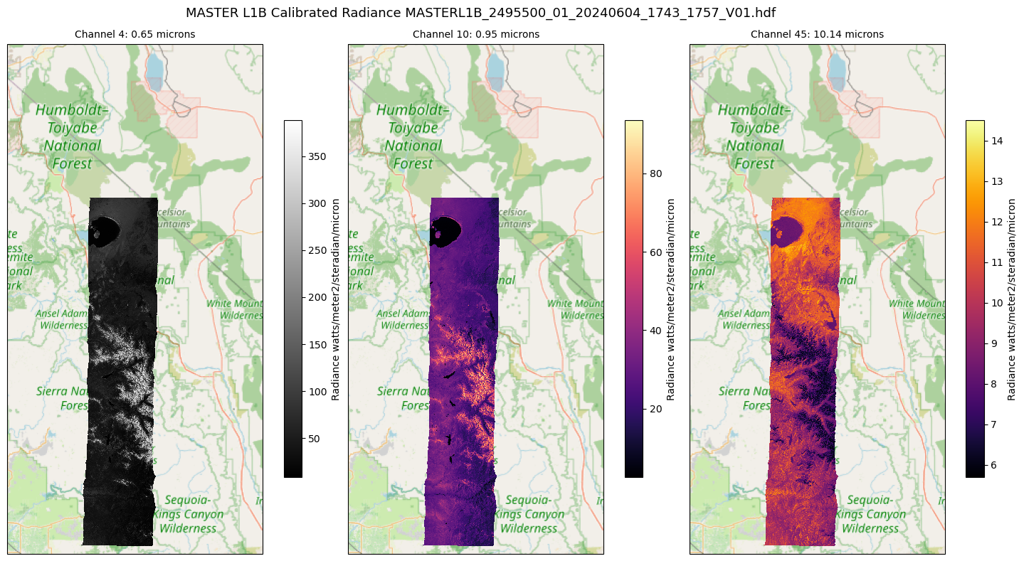

References¶

Hook, S. J., Myers, J. S., Thome, K. J., Fitzgerald, M., Kahle, A. B., Airborne Sensor Facility NASA Ames Research Center, & Green, R. O. (2024). MASTER: Western Diversity Time Series Campaign, WDTS, Spring 2024. ORNL Distributed Active Archive Center. 10.3334/ORNLDAAC/2383