
NASA Earthdata Search and Discovery of Airborne AVIRIS Data#
Summary
This notebook will demonstrate how to search, discover, subset, and access NASA airborne imaging spectrometer data derived from the AVIRIS (Airborne Visible / Infrared Imaging Spectrometers) suite of instruments. AVIRIS data are archived to NASA Earthdata collections, but but given the many years of flights in support of varied NASA campaigns, can be a challenge to discover and access.
The earthaccess Python library simplifies programmatic discovery and access of NASA Earthdata data including the many AVIRIS instrument’s radiance, reflectance, and further derived campaign data. earthaccess is a useful Python library that facilitates finding and downloading or streaming data over HTTPS or s3. earthaccess searches NASA’s Common Metadata Repository (CMR) which is a metadata system that catalogs Earth Science data and associated metadata records. This can then be used to download granules or generate lists of granule search result URLs.
With areas and times of interest identified, flight metadata will be used to build and visual flight paths within those subset parameters.
Background
Developed at the NASA Jet Propulsion Laboratory (JPL), the Airborne Visible / Infrared Imaging Spectrometers (AVIRIS) are a unique suite of optical sensors that collect data while mounted on airborne platforms such as the B200 LARC or an ER-2 AFRC. Imaging spectrometers collect light reflected off of an object (the Earth in this case) and then analyze the intensity of the wavelengths present at each pixel. As their names suggest, the AVIRIS instruments collect light in the visible to infrared wavelenths. These data can be used for characterization of the Earth’s surface and atmosphere and applied to studies in the fields of oceanography, environmental science, snow hydrology, geology, volcanology, soil and land management, atmospheric and aerosol studies, agriculture, and limnology.
Green, R.O., M.L. Eastwood, C.M. Sarture, T. G. Chrien, M. Aronsson, B.J. Chippendale, J.A. Faust, B.E. Pavri, C. J. Chovit, M. Solis, M.R. Olah, and O. Williams. 1998. Imaging Spectroscopy and the Airborne Visible/Infrared Imaging Spectrometer (AVIRIS). Remote Sensing of Environment 65:227- 248. https://doi.org/10.1016/S0034-4257(98)00064-9
Chadwick KD, Brodrick PG, Grant K, et al. Integrating airborne remote sensing and field campaigns for ecology and Earth system science. Methods Ecol Evol. 2020; 11: 1492–1508. https://doi.org/10.1111/2041-210X.13463
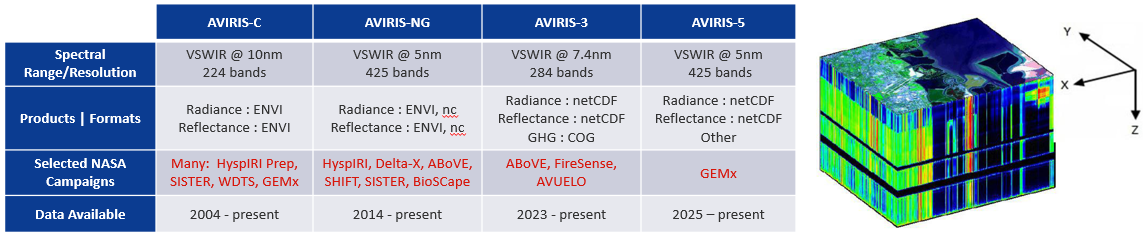
AVIRIS imaging spectrometers break down light into hundreds of narrow spectral bands, providing a spectrum for each point (or pixel) in the image. The resulting data are typically stored in a 3-dimensional array sometimes referred to as a data cube. The x and y dimensions represent the spatial dimensions of the image and the z dimension represents the wavelength information. JPL processes and provides data as radiance (L1B) and reflectance (L2A) which are archived and publically available through NASA Earthdata Facility Instrument Collections. These data files are historically distributed in a popular remote sensing ENVI file format and more recently as a standardized netCDF file format.
AVIRIS Data Processing Levels
Level |
Description |
|---|---|
L1B |
Resampled calibrated data in units of spectral radiance as well as observational geometry and illumination parameters |
L2 |
Calibrated Reflectance |
L2A |
Orthocorrected and atmospherically corrected reflectance data |
L2B |
Enhanced Surface Reflectance which can include topographic, glint, and bidirectional reflectance distribution function (BRDF) corrections |
L3 |
Variables are mapped on uniform space-time grid scales, usually with some completeness and consistency |
NASA Earthdata AVIRIS Project Data
Facility Instrument Links
AVIRIS-Classic: L1B Calibrated Radiance, Facility Instrument Collection, V1
AVIRIS-Classic: L2 Calibrated Reflectance, Facility Instrument Collection, V1
AVIRIS-NG L1B Calibrated Radiance, Facility Instrument Collection, V1
AVIRIS-NG L2 Surface Reflectance, Facility Instrument Collection, V1
AVIRIS-3 L1B Calibrated Radiance, Facility Instrument Collection
AVIRIS-3 L2A Orthocorrected Surface Reflectance, Facility Instrument Collection
Notebook Requirements
A NASA Earthdata Login account is required
Learning Objectives
login and authenticate to NASA Earthdata Login using earthaccess
construct searches of the NASA Common Metadata Repository (CMR) for specific airborne instruments
construct searches of the NASA Common Metadata Repository (CMR) for specific NASA Projects/Campaigns
narrow a search of the CMR to for files from AVIRIS instrument flights based on a spatial area of interest
programmatically discover specific AVIRIS- file access URLs based on metadata and spatial/temporal parameters
create flight line bounding boxes from a search result using CMR file(granule)-level metadata
Set Up#
Import the required Python libraries
import earthaccess
import geopandas as gpd
import pyproj
from pyproj import Proj
import xarray as xr
import matplotlib.pyplot as plt
import numpy as np
import pandas as pd
from shapely.ops import transform
from shapely.ops import orient
from shapely.geometry import Polygon, MultiPolygon
import folium

earthaccess is a Python library that simplifies data discovery and access to NASA Earthdata data by providing an abstraction layer to NASA’s APIs for programmatic access.
earthaccess will be used to:
Authentication:- handles a user’s identity (authentication) with NASA’s Earthdata Login (EDL),Search:search the NASA Earthdata Data holdings using NASA’s Common Metadata Repository (CMR), andAccess:provide direct cloud file download and access
Earthdata Login
NASA Earthdata Login is a user registration and profile management system for users getting Earth science data from NASA Earthdata. If you download or access NASA Earthdata data, you need an Earthdata Login.
Authentication#
Using earthaccess we’ll login and authenticate to NASA Systems.
For this exercise, we will be prompted for and interactively enter our Eathdata Login credentials (login, password)
auth = earthaccess.login()
Searching by Collection#
The earthaccess search_datasets function with the keyword argument can be used to search collections.
Given the many Instruments and Campaigns, there are several AVIRIS-* collections or datasets available within the NASA Earthdata cloud archive.
# Retrieve Collections
collections = earthaccess.search_datasets(keyword='AVIRIS')
# Print Quantity of Results
print(f'Collections found: {len(collections)}')
Printing the collections object explores all of the json metadata.
#Print collections
#printing the first index
#collections[0]
We can create a list of the short-name, concept-id, version, and EntryTitle of each result collection using list comprehension. These fields are important for specifying and searching for data within collections.
collections_info = [
    {
        'short_name': c.summary()['short-name'],
        'collection_concept_id': c.summary()['concept-id'],
        'version': c.summary()['version'],
        'entry_title': c['umm']['EntryTitle']
    }
    for c in collections
]
pd.set_option('display.max_colwidth', 150)
collections_info = pd.DataFrame(collections_info)
collections_info
Searching by Instrument#
#instrument = earthaccess.search_datasets(instrument="AVIRIS-3")
instrument = earthaccess.search_datasets(instrument="AVIRIS-NG")
#instrument = earthaccess.search_datasets(instrument="AVIRIS") # AVIRIS-Classic
print(f"Total Datasets (instrument) found: {len(instrument)}")
instrument_info = [
    {
        'short_name': i.summary()['short-name'],
        'collection_concept_id': i.summary()['concept-id'],
        'version': i.summary()['version'],
        'entry_title': i['umm']['EntryTitle']
    }
    for i in instrument
]
pd.set_option('display.max_colwidth', 150)
instrument_info = pd.DataFrame(instrument_info)
instrument_info
The collection concept-id or short_name are unique to each collection. After finding the collection you want to search, you can use the short_name or concept-id to search for granules (or files) within that collection.
Searching by Project#
results = earthaccess.search_datasets(project="BioSCape")
#results = earthaccess.search_datasets(project="ABoVE")
print(f"Total Datasets (results_projects) found: {len(results)}")
for item in results:
    summary = item.summary()
    print(summary["short-name"])
Search AVIRIS-3 Instrument (only) for Specific Project/Campaign#
AVIRIS-3 datasets contain
campaigninformation at the granule level within the Unified Metadata Model-Granule (UMM-G)AdditionalAttributesFor AVIRIS-3 L1B data, this next code block lists the campaigns and number of granules in each campaign
Note that at the time of writing this Notebook, this functionality is specific to AVIRIS-3 Datasets
def  get_campaign_names(granules):
    """get campaign names for all granules"""
    c = []
    for g in granules:
        for attrs in vars(g)['render_dict']['umm']['AdditionalAttributes']:
            if attrs['Name'] == 'Campaign':
                c += attrs['Values']
    return c

# earthdata search
granules = earthaccess.search_data(
    short_name = 'AV3_L1B_RDN_2356',
    #doi="10.3334/ORNLDAAC/2356"
)

campaigns = get_campaign_names(granules)

#print campaign names and granules
for name in list(set(campaigns)):
    print(f'{name} --> {campaigns.count(name)} granules')
If you know a NASA Project or Campaign employed the AVIRIS-3 instrument, you can directly query the AdditionalAttributes
#doi="10.3334/ORNLDAAC/2356" # AV3_L1B_RDN_2356
short_name = "AV3_L1B_RDN_2356"
query = earthaccess.DataGranules().short_name(short_name)
query.params['attribute[]'] = 'string,Campaign,SHIFT'
l1b = query.get_all()
print(f'Granules found: {len(l1b)}')
Setting Search Parameters for Granules#
We’ll use a NEON AOP Flight Boundary to search for AVIRIS data in a spatial area of interest.
NEON AOP Flight Boundaries [https://hub.arcgis.com/datasets/f27616de7f9f401b8732cdf8902ab1d8/about]
# read the AVIRIS-NG_flights.shp file and convert to geojson using geopandas
AOP_polys = gpd.read_file('~/shared-public/data/AOP_Flightboxes.shp')
AOP_polys.to_file('aop_json.geojson', driver='GeoJSON')
gdf = gpd.read_file('aop_json.geojson')

# Access the CRS using the .crs attribute
if gdf.crs:
    print(f"CRS: {gdf.crs}")
gdf.explore()
serc_aop = gdf[(gdf['siteID'] == 'SJER') & (gdf['priority'] == 1)]
#serc_aop = gdf[(gdf['siteID'] == 'BARR') & (gdf['priority'] == 1)]
print(serc_aop.head())
serc_aop.explore()
Use the NEON AOP Boundary file to search for AVIRIS-Classic L2 Reflectance data within that boundary
# bounding lon, lat as a list of tuples
bounds = serc_aop.geometry.apply(orient, args=(1,))
bounds
# simplifying the polygon to bypass the coordinates
# limit of the CMR with a tolerance of .01 degrees
xy = bounds.simplify(0.01).get_coordinates()
print(xy)

date_range = ("2019-01-01", "2019-12-31")

results = earthaccess.search_data(
    short_name = 'AVIRIS-Classic_L2_Reflectance_2154',
    #short_name = 'ABoVE_Airborne_AVIRIS_NG_V3_2362',
    #short_name = 'AVIRIS-NG_L2_Reflectance_2110	',
    #short_name = 'AVIRIS-NG_L1B_radiance_2095',
    polygon=list(zip(xy.x, xy.y)),
    temporal = date_range
)
print(f"Total AVIRIS collections found: {len(results)}")
For our search parameters, let’s explore the granules found
Let’s look at the first result
results[:1]
results[0]
You can download these files directly to your local machine by clicking on any of the files
We also see that these data are Cloud Hosted: True
Create and Visualize the Bounding Boxes of the subset of files#
From each granule, we’ll use the CMR Geometry information to create a plot of the AVIRIS-3 flight lines from our temporal and spatial subset
Below, we define two functions to plot the search results over a basemap
Function 1: converts UMM geometry to multipolygons –
UMMstands for NASA’s Unified Metadata ModelFunction 2: converts the Polygon List [ ] to a
geopandasdataframe
def convert_umm_geometry(gpoly):
    """converts UMM geometry to multipolygons"""
    multipolygons = []
    for gl in gpoly:
        ltln = gl["Boundary"]["Points"]
        points = [(p["Longitude"], p["Latitude"]) for p in ltln]
        multipolygons.append(Polygon(points))
    return MultiPolygon(multipolygons)
def convert_list_gdf(datag):
    """converts List[] to geopandas dataframe"""
    # create pandas dataframe from json
    df = pd.json_normalize([vars(granule)['render_dict'] for granule in datag])
    # keep only last string of the column names
    df.columns=df.columns.str.split('.').str[-1]
    # convert polygons to multipolygonal geometry
    df["geometry"] = df["GPolygons"].apply(convert_umm_geometry)
    # return geopandas dataframe
    return gpd.GeoDataFrame(df, geometry="geometry", crs="EPSG:4326")

subset_gdf = convert_list_gdf(results)
subset_gdf.crs
#subset_gdf.explore()

subset_gdf = convert_list_gdf(results)
subset_gdf.drop('Version', axis=1, inplace=True)
subset_gdf.explore(fill=False, tiles='https://mt1.google.com/vt/lyrs=s&x={x}&y={y}&z={z}', attr='Google')
#subset_gdf.explore()

subset_gdf = convert_list_gdf(results)
subset_gdf.drop('Version', axis=1, inplace=True)

# Create the base map with `serc_aop`
base_map = serc_aop.explore(
    color="red",  # Outline color for serc_aop features
    fill=False,   # No fill for serc_aop
    legend=True,  # Display legend for serc_aop
    tiles='https://mt1.google.com/vt/lyrs=s&x={x}&y={y}&z={z}',  # Google Satellite tiles
    attr='Google'
)

# Add `subset_gdf` layer to the base map
final_map = subset_gdf.explore(
    color="blue",  # Outline color for subset_gdf features
    fill=False,    # No fill for subset_gdf
    legend=True,   # Display legend for subset_gdf
    m=base_map     # Add this layer to the base map
)

# Display the map
final_map